
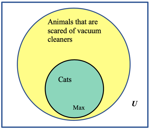
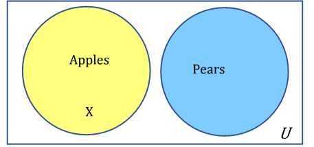
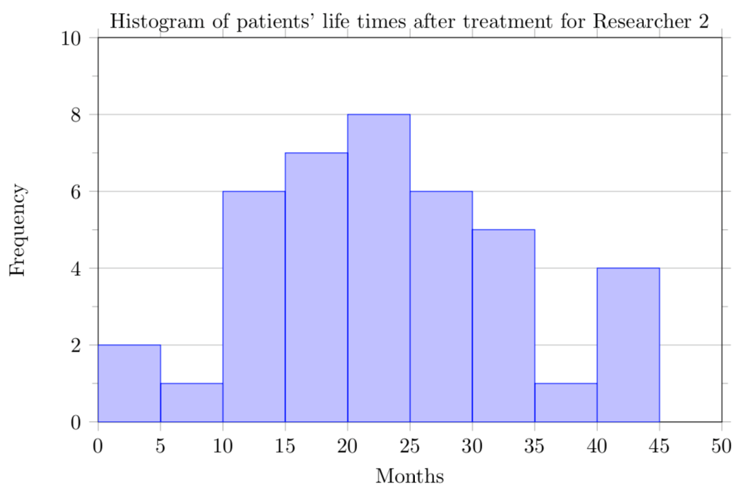
1.1.11.1.
Solution.
- Proposition
- Not a proposition
- Proposition
- Proposition
| A | B | A and B |
|---|---|---|
| T | T | T - I live in Oregon and I go to PCC |
| T | F | F - I live in Oregon and I don’t go to PCC |
| F | T | F - I don’t live in Oregon and I go to PCC |
| F | F | F - I don’t live in Oregon and I don’t go to PCC |
| A | B | Not B | A and not B |
|---|---|---|---|
| T | T | F | F |
| T | F | T | T |
| F | T | F | F |
| F | F | T | F |
| A | B | C | A and B and C | Not (A and B and C) |
|---|---|---|---|---|
| T | T | T | T | F |
| T | T | F | F | T |
| T | F | T | F | T |
| T | F | F | F | T |
| F | T | T | F | T |
| F | T | F | F | T |
| F | F | T | F | T |
| F | F | F | F | T |
| A | B | C | A and B | Not (A and B) | Not (A and B) or C |
|---|---|---|---|---|---|
| T | T | T | T | F | T |
| T | T | F | T | F | F |
| T | F | T | F | T | T |
| T | F | F | F | T | T |
| F | T | T | F | T | T |
| F | T | F | F | T | T |
| F | F | T | F | T | T |
| F | F | F | F | T | T |
| A | B | C | A and B | If (A and B), then C |
|---|---|---|---|---|
| T | T | T | T | T |
| T | T | F | T | F |
| T | F | T | F | T |
| T | F | F | F | T |
| F | T | T | F | T |
| F | T | F | F | T |
| F | F | T | F | T |
| F | F | F | F | T |
| A | C | A and C | Not A | If (A and C), then not A |
|---|---|---|---|---|
| T | T | T | F | F |
| T | F | F | F | T |
| F | T | F | T | T |
| F | F | F | T | T |
=4/7 which gives approximately 0.571429=8+19 which gives 27=12*9 which gives 108=8^3 which gives 512=7.50/44.50 which gives approximately 0.1685, or approximately 16.85%=5780.23-5250 which gives $530.23=530.23/5250 which gives approximately 0.100996, or approximately 10.1%=5250*115.5% which gives exactly $6063.75=1000*103%*103% which gives $1060.90=1000*(103%)^2 gives the same result of $1060.90, because raising 103% to the second power means the same as multiplying 103% by itself two times.=1000*(103%)^15 which gives $1557.97 rounded to the nearest cent= B2*103% and the remaining cells are computed using the fill down feature.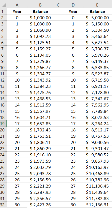
=FV(0.07/52,52*20,0,1000)
=FV(0.05/1,1*10,0,300)
=FV(0.04/52,52*25,0,10000)
=PV(0.05/4,4*4,0,20000)
=EFFECT(0.0375,12) \(=3.82\%\) and Ted =EFFECT(0.038,1) =3.8%. Bill has an effective rate of 3.82% and Ted has a rate of 3.8%.=FV(0.0375/12,5*12,0,6700)
=FV(0.038,5,0,6500)
2500*EXP(0.04*10)
=5000*EXP(0.045*5)
FV(0.065/12,12*35,250)
=FV(0.0775/4,4*30,750)
=FV(0.09/12,12*5,130)
=FV(0.09/12,12*25,0,9805.14)=PMT(0.038/12,30,0,3500)=PMT(0.06/12,12*30,0,450000)
=FV(0.056/12,12*25,0,55000)
=FV(0.056/12,12*25,375)
=FV(0.045/12,12*10,100,1000)
=FV(0.04/12,12*25,100)
=FV(0.04/12,12*40,100=FV(0.035/52,52*18,50)
=PV(0.035/52,52*18,0,65164.37)
=PV(0.055/12,12*30,-700) [Note 700 is entered as negative, to signify a payment]=PMT(0.02/12,48,25000)
=PMT(0.05/12,12*30,180000)
=PMT(0.06/12,12*30,180000)
=PMT(0.03/12,12*5,24000)
=PV(0.03/12,12*2,-431.25)
=PV(0.04/12,12*30,950) which gives $198,988.18.=PMT(0.05,10,100000,0) which gives $12,950.46.=PMT(0.045/12,12*30,250000) which gives $1,266.71.=PV(0.045/12,12*20,1266.71) which gives $200,223.07.=PV(0.045/12,12*10,1266.71) which gives $122,223.99.=FV(0.035/12,3*12,200,0) = $7,579.95. Paul will have $7,579.95 in 3 years.=PV(0.028/12,4*12,100,0) = $4,535.96. Miao can finance $4,535.96 in equipment to have a monthly loan payment of $100 for 4 years.=PMT(0.043/12,30*12,364500,0) = $1,803.81. Their mortgage payment would be $1,803.81.=FV(0.048/12,20*12,150,0) = $60,251.26. Zahid would have $60,251.26 if he puts in $150 per month for 20 years.=FV(0.048/12,10*12,300,0) = $46,089.59. Zahid would only have $46,089.59 if he waited and put in $300 per month for 10 years.=FV(0.056/4, 4*14, 0, 1525)
=FV(0.056/52, 52*14, 0, 1525)
=1525*EXP(0.056*14)
=FV(0.065/4, 4*15, 0, 25000)
=FV(0.065/12, 12*25, 350, 0)
=FV(0.065/4, 4*15, 500, 0)
=FV(0.045/52, 52*30, 75, 0)
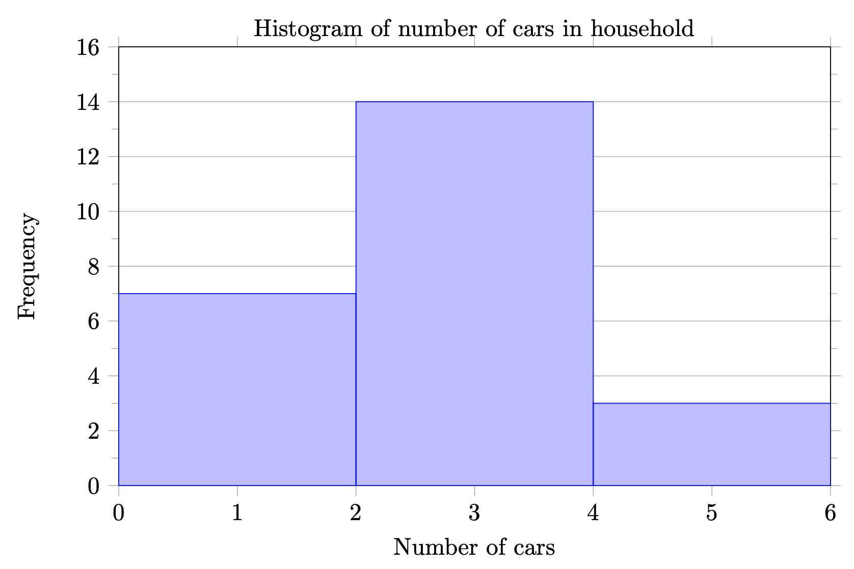
| Number of cars in household |
Frequency |
|---|---|
| 0-1 | 7 |
| 2-3 | 14 |
| 4-5 | 3 |
=average(7.50,25,10,10,7.50,8.25,9,5,15,8,7.25,7.50,8,7,12)=median(7.50,25,10,10,7.50,8.25,9,5,15,8,7.25,7.50,8,7,12)=average(15.2,18.8,19.3,19.7,20.2,21.8,22.1,29.4)=median(15.2,18.8,19.3,19.7,20.2,21.8,22.1,29.4)=average(A1:A40)=median(A1:A40)=average(A1:A40)=median(A1:A40)
| 0, | 0, | 0, | 0, | 10 |
| 0, | 0, | 2, | 4, | 4 |
| 0, | 1, | 1, | 1, | 7 |
| 10, | 10, | 10, | 10, | 10 |
| 0, | 0, | 10, | 15, | 20 |
| 1, | 5, | 10, | 10, | 10 |
| Data Value | Deviation | Deviation Squared |
|---|---|---|
| \(7.5\) | \(7.5-9.8=-2.3\) | \((-2.3)^2=5.29\) |
| \(25\) | \(25-9.8=15.2\) | \((15.2)^2=231.04\) |
| \(10\) | \(10-9.8=0.2\) | \((0.2)^2=0.04\) |
| \(10\) | \(10-9.8=0.2\) | \((0.2)^2=0.04\) |
| \(7.5\) | \(7.5-9.8=-2.3\) | \((-2.3)^2=5.29\) |
| \(8.25\) | \(8.25-9.8=-1.55\) | \((-1.55)^2=2.4\) |
| \(9\) | \(9-9.8=-0.8\) | \((-0.8)^2=0.64\) |
| \(5\) | \(5-9.8=-4.8\) | \((-4.8)^2=23.04\) |
| \(15\) | \(15-9.8=5.2\) | \((5.2)^2=27.04\) |
| \(8\) | \(8-9.8=-1.8\) | \((-1.8)^2=3.24\) |
| \(7.25\) | \(7.25-9.8=-2.55\) | \((-2.55)^2=6.5\) |
| \(7.5\) | \(7.5-9.8=-2.3\) | \((-2.3)^2=5.29\) |
| \(8\) | \(8-9.8=-1.8\) | \((-1.8)^2=3.24\) |
| \(7\) | \(7-9.8=-2.8\) | \((-2.8)^2=7.84\) |
| \(12\) | \(12-9.8=2.2\) | \((2.2)^2=4.84\) |
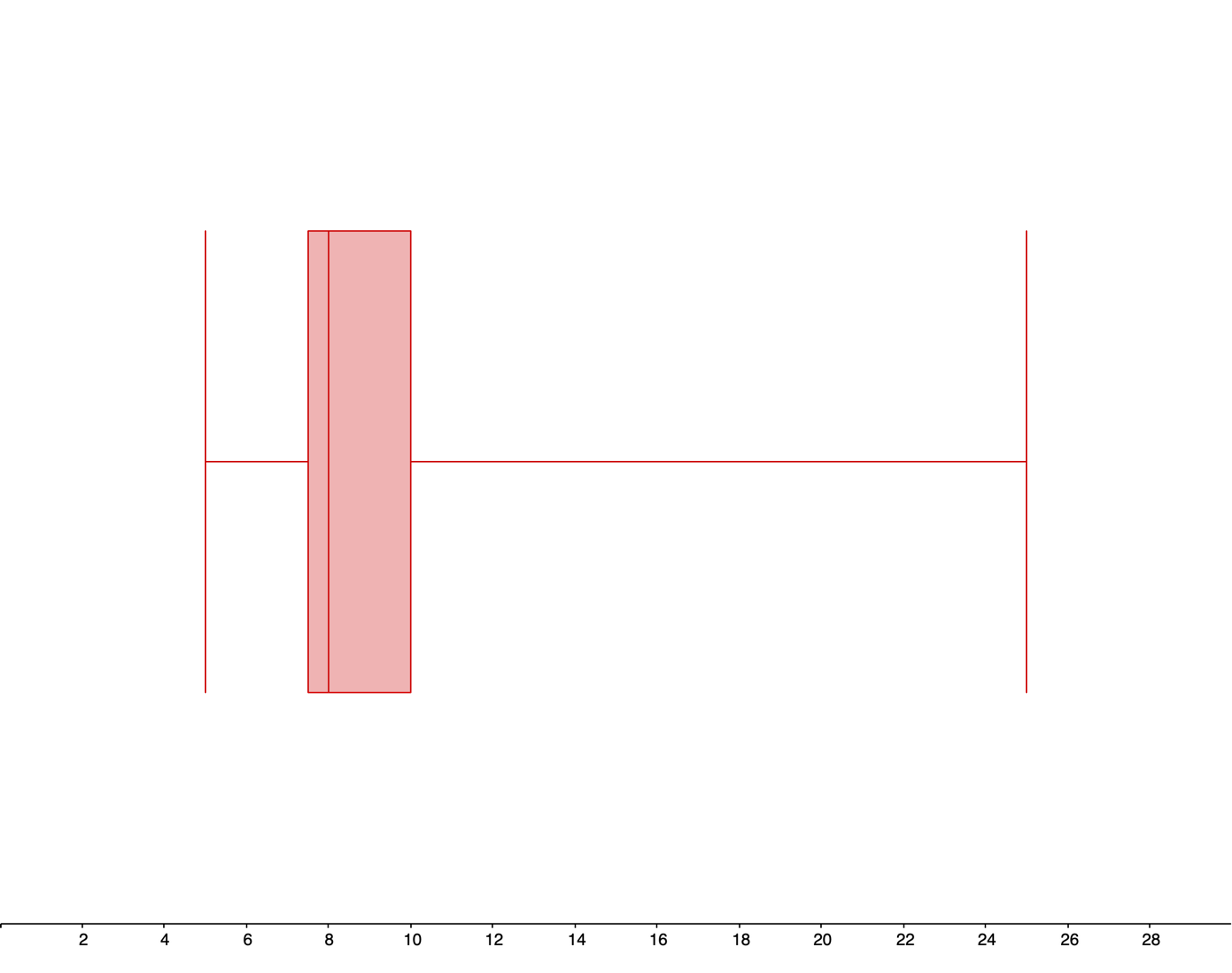
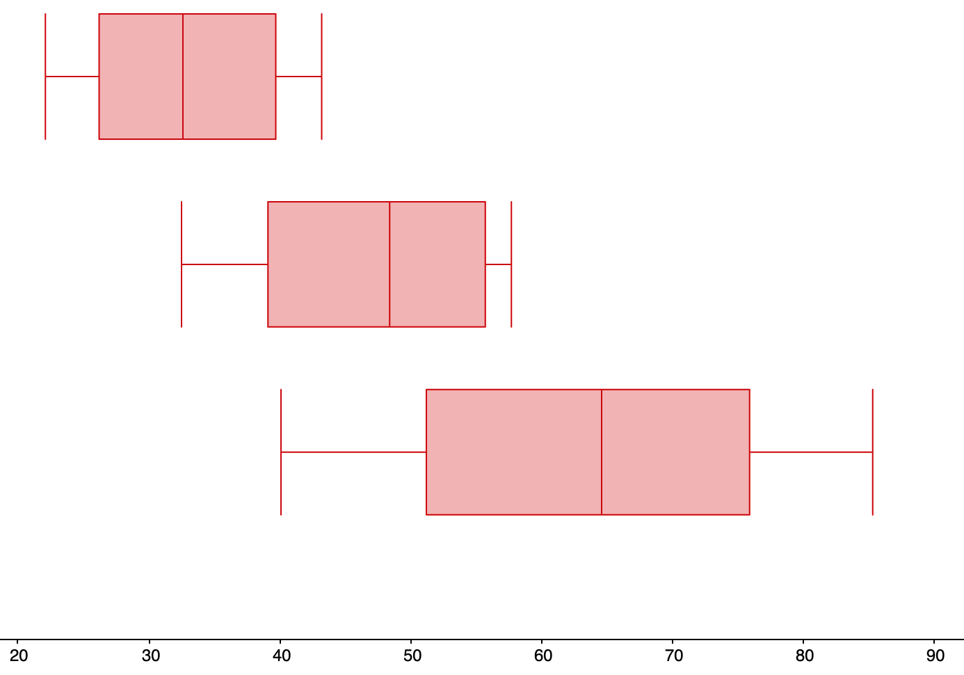
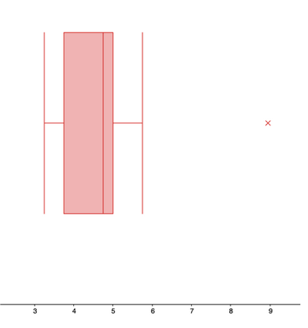
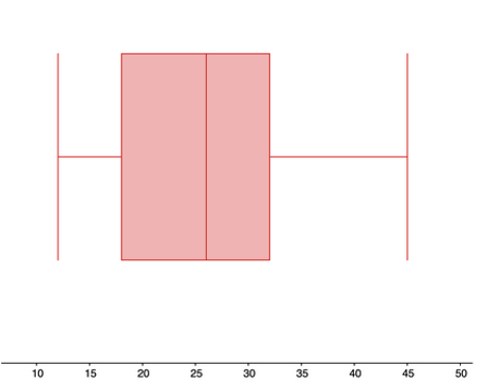
| Min | Q1 | Median | Q3 | Max |
|---|---|---|---|---|
| $5 | $7.50 | $8 | $10 | $25 |
| Min | Q1 | Median | Q3 | Max |
|---|---|---|---|---|
| $5 | $7.50 | $8 | $10 | $25 |
| Min | Q1 | Median | Q3 | Max |
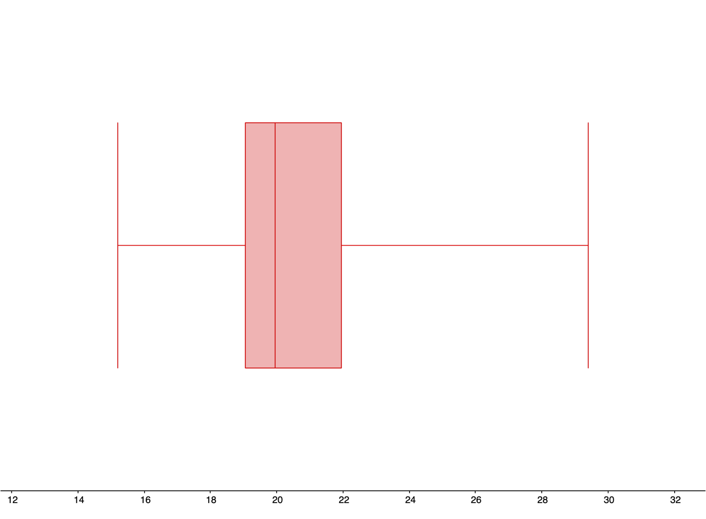
|---|---|---|---|---|
| 15.2 seconds | 19.05 seconds | 19.95 seconds | 21.95 seconds | 29.4 seconds |
| Min | Q1 | Median | Q3 | Max |
|---|---|---|---|---|
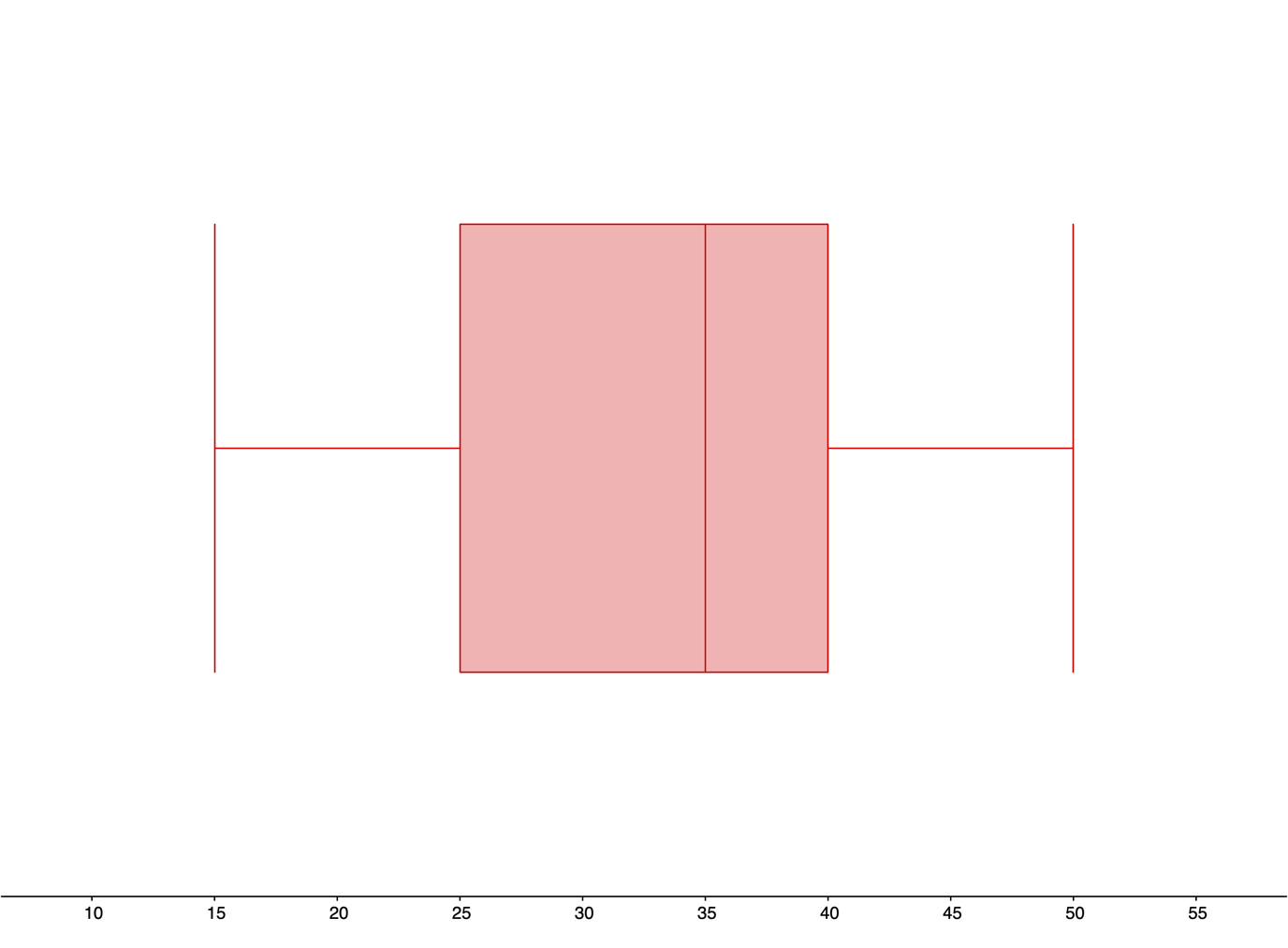
| 15 thousand dollars |
25 thousand dollars |
35 thousand dollars |
40 thousand dollars |
50 thousand dollars |
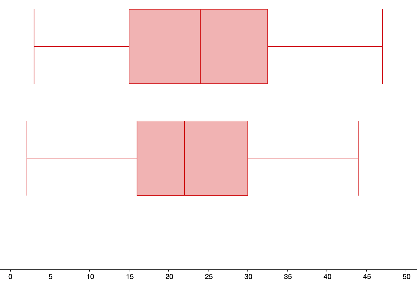
| Min | Q1 | Median | Q3 | Max |
|---|---|---|---|---|
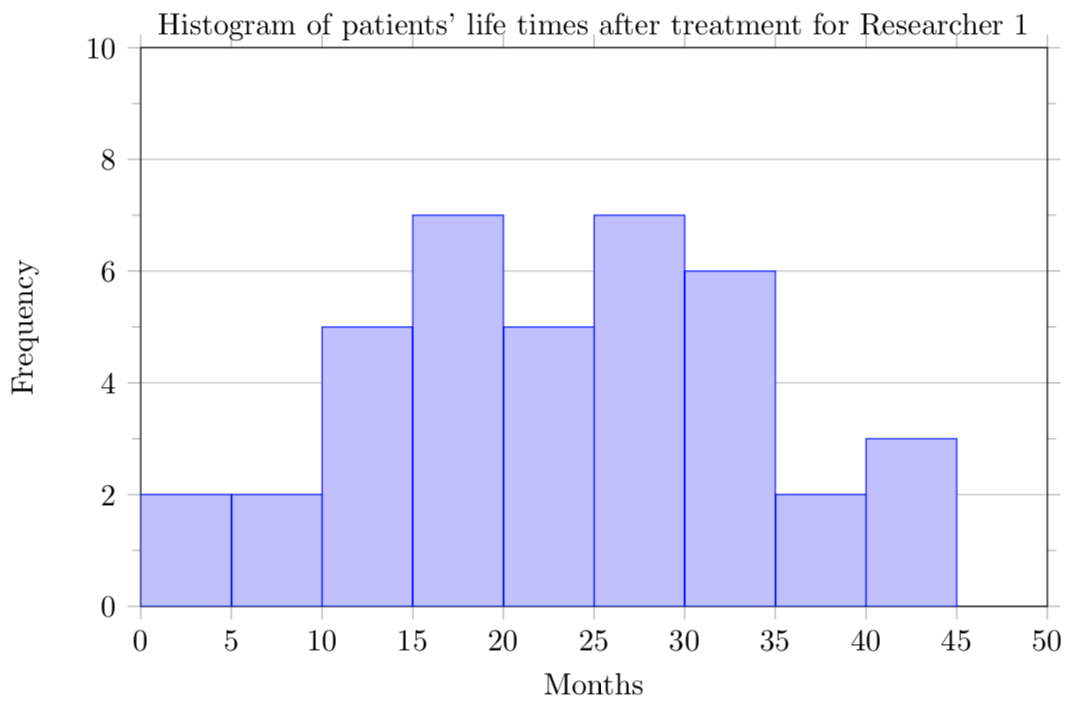
| 3 months | 15 months | 24 months | 32.5 months | 47 months |
| Min | Q1 | Median | Q3 | Max |
|---|---|---|---|---|
| 2 months | 16 months | 22 months | 30 months | 44 months |
| Min | Q1 | Median | Q3 | Max |
|---|---|---|---|---|
| 22.1 chess pieces |
26.2 chess pieces |
32.6 chess pieces |
39.7 chess pieces |
43.2 chess pieces |
| Min | Q1 | Median | Q3 | Max |
|---|---|---|---|---|
| 32.5 chess pieces |
39.1 chess pieces |
48.4 chess pieces |
55.7 chess pieces |
57.7 chess pieces |
| Min | Q1 | Median | Q3 | Max |
|---|---|---|---|---|
| 40.1 chess pieces |
51.2 chess pieces |
64.6 chess pieces |
75.9 chess pieces |
85.3 chess pieces |
| Min | Q1 | Median | Q3 | Max |
|---|---|---|---|---|
| $3.25 | $3.75 | $4.75 | $5.00 | $8.95 |
| Min | Q1 | Median | Q3 | Max |
|---|---|---|---|---|
| $12 thousand | $18 thousand | $26 thousand | $32 thousand | $45 thousand |
| Food Insecure | Not Food Insecure | Total | |
|---|---|---|---|
| Housing Insecure | 380 | 60 | 440 |
| Not Housing Insecure | 300 | 460 | 760 |
| Total | 680 | 520 | 1200 |
| Breakfast | No Breakfast | Total | |
|---|---|---|---|
| Floss | 12 | 49 | 61 |
| No Floss | 3 | 8 | 11 |
| Total | 15 | 57 | 72 |
| A | Not A | Total | |
|---|---|---|---|
| B | 10 | 20 | 30 |
| Not B | 20 | 25 | 45 |
| Total | 30 | 45 | 75 |
| Game/Software | No Game/Software | Total | |
|---|---|---|---|
| Computer | 10% | 5% | 15% |
| No Computer | 15% | 70% | 85% |
| Total | 25% | 75% | 100% |
| Hardcover | Paperback | Total | |
|---|---|---|---|
| Fiction | 13 | 59 | 72 |
| Nonfiction | 15 | 8 | 23 |
| Total | 28 | 67 | 95 |
| Die roll | Gold | Silver | Black |
|---|---|---|---|
| Outcome | $3 | $2 | -$1> |
| Probability | \(3/37\) | \(6/37\) | \(28/37\) |
| Die roll outcome | 1, 2, 3, or 4 | 5 | 6 |
|---|---|---|---|
| Outcome | $5 | $0 | -$2 |
| Probability | \(1/6\) | \(1/6\) | \(4/6\) |
| Type | Channel 2 | Channel 6 | Channel 8 | Channel 12 | Total |
|---|---|---|---|---|---|
| Drama | 5 | 2 | 4 | 4 | 15 |
| Sitcom | 6 | 9 | 7 | 3 | 25 |
| Game Show | 4 | 4 | 3 | 4 | 15 |
| News | 3 | 2 | 2 | 3 | 10 |
| Total | 18 | 17 | 16 | 14 | 65 |
| Color | Black | Orange | Yellow |
|---|---|---|---|
| x | $3 | $2 | -$1 |
| P(x) | \(2/26\) | \(4/26\) | \(20/26\) |
| Outcome | Product Failed | Didn’t Fail |
|---|---|---|
| x | -$450 | $0 |
| P(x) | 0.015 | 0.985 |
| Number of voters | 3 | 3 | 1 | 3 | 2 |
|---|---|---|---|---|---|
| 1st choice | A | A | B | B | C |
| 2nd choice | B | C | A | C | A |
| 3rd choice | C | B | C | A | B |
| State | Population | Number of Representatives |
Number of Senators |
Number of Electors |
|---|---|---|---|---|
| Gandhi | 450,000 | 9 | 2 | 11 |
| Mandela | 150,000 | 3 | 2 | 5 |
| Gbowee | 600,000 | 12 | 2 | 14 |
| Total | 1,200,000 | 24 | 6 | 30 |
| State | Population | Number of Representatives |
Number of Senators |
Number of Electors |
|---|---|---|---|---|
| Tamez | 280,000 | 7 | 2 | 9 |
| Teters | 200,000 | 5 | 2 | 7 |
| Herrington | 400,000 | 10 | 2 | 12 |
| Osawa | 360,000 | 9 | 2 | 11 |
| Total | 1,240,000 | 31 | 8 | 39 |
| State | Votes for Candidate A |
Votes for Candidate B |
Number of Electoral Votes for A |
Number of Electoral Votes for B |
|---|---|---|---|---|
| Gandhi | 216,000 | 234,000 | 0 | 11 |
| Mandela | 37,500 | 112,500 | 0 | 5 |
| Gbowee | 489,450 | 110,550 | 14 | 0 |
| Total Votes | 742,950 | 457,050 | 14 | 16 |
| State | Votes for Candidate A |
Votes for Candidate B |
Number of Electoral Votes for A |
Number of Electoral Votes for B |
|---|---|---|---|---|
| Tamez | 95,480 | 184,250 | 0 | 9 |
| Teters | 104,200 | 95,800 | 7 | 0 |
| Herrington | 203,600 | 196,400 | 12 | 0 |
| Osawa | 46,080 | 313,920 | 0 | 11 |
| Total Votes | 449,360 | 790,640 | 19 | 20 |
| State | Population | Number of Representatives |
Number of Senators |
Number of Electors |
Electoral Votes per 50,000 people |
|---|---|---|---|---|---|
| Gandhi | 450,000 | 9 | 2 | 11 | 1.22 |
| Mandela | 150,000 | 3 | 2 | 5 | 1.67 |
| Gbowee | 600,000 | 12 | 2 | 14 | 1.17 |
| State | Population | Number of Representatives |
Number of Senators |
Number of Electors |
Electoral Votes per 50,000 people |
|---|---|---|---|---|---|
| Tamez | 280,000 | 7 | 2 | 9 | 1.29 |
| Teters | 200,000 | 5 | 2 | 7 | 1.40 |
| Herrington | 400,000 | 10 | 2 | 12 | 1.20 |
| Osawa | 360,000 | 9 | 2 | 11 | 1.22 |
| District | D Votes | R Votes | D Surplus Votes | R Surplus Vote |
|---|---|---|---|---|
| 1 | 1 | 6 | 1 | \(6-4=2\) |
| 2 | 3 | 4 | 3 | \(4-4=0\) |
| 3 | 6 | 1 | \(6-4=2\) | 1 |
| 4 | 7 | 0 | \(7-4=3\) | 0 |
| Total | 17 | 11 | 9 | 3 |
| District | D Votes | R Votes | D Surplus Votes | R Surplus Vote |
|---|---|---|---|---|
| 1 | 2 | 3 | 2 | \(3-3=0\) |
| 2 | 2 | 3 | 2 | \(3-3=0\) |
| 3 | 2 | 3 | 2 | \(3-3=0\) |
| 4 | 4 | 1 | \(4-3=1\) | 1 |
| 5 | 2 | 3 | 2 | \(3-3=0\) |
| Total | 12 | 13 | 9 | 1 |
| District | D Votes | R Votes | D Surplus Votes | R Surplus Vote |
|---|---|---|---|---|
| 1 | 2 | 7 | 2 | \(7-5=2\) |
| 2 | 5 | 4 | \(5-5=0\) | 4 |
| 3 | 2 | 7 | 2 | \(7-5=2\) |
| 4 | 5 | 4 | \(5-5=0\) | 4 |
| 5 | 4 | 5 | 4 | \(5-5=0\) |
| Total | 18 | 27 | 8 | 12 |
| District | D Votes | R Votes | D Surplus Votes | R Surplus Vote |
|---|---|---|---|---|
| 1 | 3 | 2 | \(3-3=0\) | 2 |
| 2 | 3 | 2 | \(3-3=0\) | 2 |
| 3 | 3 | 2 | \(3-3=0\) | 2 |
| 4 | 3 | 2 | \(3-3=0\) | 2 |
| 5 | 3 | 2 | \(3-3=0\) | 2 |
| 6 | 0 | 5 | 0 | \(5-3=2\) |
| Total | 15 | 15 | 0 | 12 |
| District | D Votes | R Votes | D Surplus Votes | R Surplus Vote |
|---|---|---|---|---|
| 1 | 2 | 7 | 2 | \(7-5=2\) |
| 2 | 2 | 7 | 2 | \(7-5=2\) |
| 3 | 9 | 0 | \(9-5=4\) | 0 |
| 4 | 2 | 7 | 2 | \(7-5=2\) |
| 5 | 1 | 8 | 1 | \(8-5=3\) |
| 6 | 4 | 5 | 4 | \(5-5=0\) |
| Total | 20 | 34 | 15 | 9 |
| State | Population | Number of Representatives |
Number of Senators |
Number of Electors |
|---|---|---|---|---|
| Fonville | 825,000 | 15 | 2 | 17 |
| Gurley | 550,000 | 10 | 2 | 12 |
| Nevarez | 275,000 | 5 | 2 | 7 |
| Total | 1,650,000 | 30 | 6 | 36 |
| State | Votes for Candidate A |
Votes for Candidate B |
Number of Electoral Votes for A |
Number of Electoral Votes for B |
|---|---|---|---|---|
| Fonville | 684,750 | 140,250 | 17 | 0 |
| Gurley | 257,400 | 292,600 | 0 | 12 |
| Nevarez | 132,275 | 142,725 | 0 | 7 |
| Total Votes | 1,074,425 | 575,575 | 17 | 19 |
| State | Population | Number of Representatives |
Number of Senators |
Number of Electors |
Electoral Votes per 55,000 people |
|---|---|---|---|---|---|
| Fonville | 825,000 | 15 | 2 | 17 | 1.13 |
| Gurley | 550,000 | 10 | 2 | 12 | 1.20 |
| Nevarez | 275,000 | 5 | 2 | 7 | 1.40 |
| District | D Votes | R Votes | D Surplus Votes | R Surplus Vote |
|---|---|---|---|---|
| 1 | 4 | 5 | 4 | \(5-5=0\) |
| 2 | 4 | 5 | 4 | \(5-5=0\) |
| 3 | 9 | 0 | \(9-5=4\) | 0 |
| 4 | 4 | 5 | 4 | \(5-5=0\) |
| 5 | 4 | 5 | 4 | \(5-5=0\) |
| Total | 25 | 20 | 20 | 0 |
