Appendix A Odd Answers

1 Logical Reasoning and Problem Solving
1.1 Logic in Everyday Life
1.1.11 Exercises

1.1.11.21.

Solution.
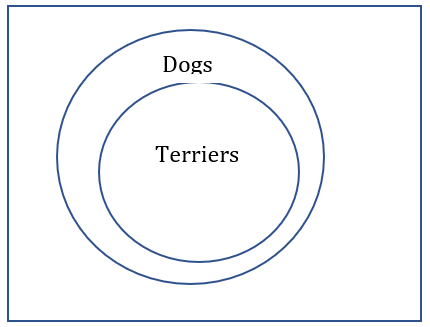
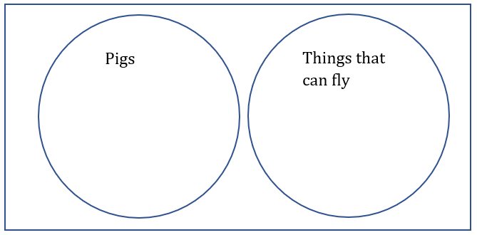
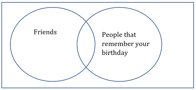
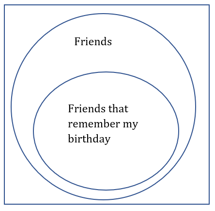
Statements i and iii are logically equivalent to each other. Statements ii and iv are logically equivalent to each other.

1.2 Sets and Venn Diagrams
1.2.12 Exercises

1.2.12.17.

Solution.
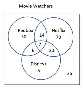
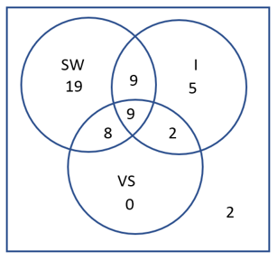
  • Region A: Unemployed non-honor-students who identify as boys
  • Region B: Unemployed honor-students who identify as boys
  • Region C: Unemployed honor-students who identify as girls or nonbinary
  • Region D: Employed non-honor-students who identify as boys
  • Region E: Employed honor-students who identify as boys
  • Region F: Employed honor-students who identify as girls or nonbinary
  • Region G: Employed non-honor-students who identify as girls or nonbinary
  • Region H: Unemployed non-honor-students who identify as girls or nonbinary

1.3 Percents
1.3.8 Exercises

1.3.8.27.

Solution.
\(\$2,000,000(1-0.095)(1+.10)=\$1,991,000.\) for a relative decrease of 0.0045 or 0.45%.

1.4 Rates and Proportions
1.4.7 Exercises

1.4.7.5.

Solution.
The 9.6-ounce container is $0.565 per ounce and the 40.3-ounce canister is $0.369 per ounce. The larger container is a better value.

1.4.7.7.

Solution.
The population density of the US is about 83.4 people per square mile. The population density of India is about 93.4 people per square mile.

1.4.7.23.

Solution.
For 5 scoops of mix you need 2.5 cups of milk. If there is no room in the cup pour it into a larger bowl and mix.

1.5 Problem Solving
1.5.6 Exercises

1.5.6.13.

Solution.
The hourly job would pay $58,740 per year. The salary of $60,000 is higher unless there is a lot of overtime pay in the hourly job.

1.5.6.15.

Solution.
It would take 30 hours of overtime in a year for the hourly pay to equal the salaried job pay.

1.5.6.17.

Solution.
It depends on the size of the party. The per person venue is less expensive up to 52 people. The per table venue is cheaper for 53 or more guests.

1.5.6.21.

Solution.
The child should get approximately 7.5 mg per day. This would be 3 of the 2.5 mg tablets.

1.6 Chapter 1 Review

1.6.19.

Solution.
The child should get approximately 300 mg per day which is 10 ml per dose or 2 teaspoons.

1.7 Truth Tables
1.7.5 Exercises

1.7.5.5.

Solution.
A B A and B
T T T - I live in Oregon and I go to PCC
T F F - I live in Oregon and I don’t go to PCC
F T F - I don’t live in Oregon and I go to PCC
F F F - I don’t live in Oregon and I don’t go to PCC

1.7.5.7.

Solution.
A B Not B A and not B
T T F F
T F T T
F T F F
F F T F

1.7.5.9.

Solution.
A B C A and B and C Not (A and B and C)
T T T T F
T T F F T
T F T F T
T F F F T
F T T F T
F T F F T
F F T F T
F F F F T

1.7.5.11.

Solution.
A B C A and B Not (A and B) Not (A and B) or C
T T T T F T
T T F T F F
T F T F T T
T F F F T T
F T T F T T
F T F F T T
F F T F T T
F F F F T T

1.7.5.13.

Solution.
A B C A and B If (A and B), then C
T T T T T
T T F T F
T F T F T
T F F F T
F T T F T
F T F F T
F F T F T
F F F F T

1.7.5.15.

Solution.
A C A and C Not A If (A and C), then not A
T T T F F
T F F F T
F T F T T
F F F T T

1.8 Describing and Critiquing Arguments
1.8.5 Exercises

1.8.5.3.

Solution.
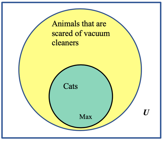
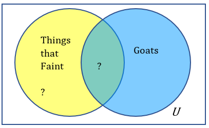
Premise: All cats are scared of vacuum cleaners.
Premise: Max is a cat.
Conclusion: Max must be scared of vacuum cleaners.
This is a deductive argument. It is valid. However, it is not sound because the premise all cats are afraid of vacuum cleaners is false. While many cats are afraid of vacuum cleaners not ALL cats are afraid. There are many videos of cats riding electronic vacuum cleaners.

1.8.5.5.

Solution.
Premise: Kiran’s female and nonbinary friends made less than Kiran’s male friends.
Conclusion: Women and nonbinary people make less than men.
This is an inductive argument. Kiran did not gather a large diverse sample because they only asked their friends. Therefore, their data has sampling bias. This makes their argument weak.

1.8.5.7.

Solution.
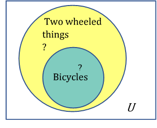
Premise: All bicycles have two wheels.
Premise: My friend’s Harley-Davidson motorcycle has two wheels.
Conclusion: It must be a bicycle.
This is a deductive argument. The argument is not valid. Based on the premises, we know that the friend’s Harley-Davidson motorcycle has two wheels, but we do not know whether or not it is a bicycle. Because it is not valid, it is also not sound.

1.8.5.9.

Solution.
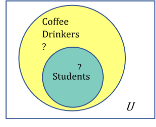
Premise: All students drink a lot of caffeine.
Premise: Brayer drinks a lot of caffeine.
Conclusion: He must be a student.
This is a deductive argument. The argument is not valid. We can not determine if Brayer is a student or not. Because it is not valid it is also not sound.

1.8.5.11.

Solution.
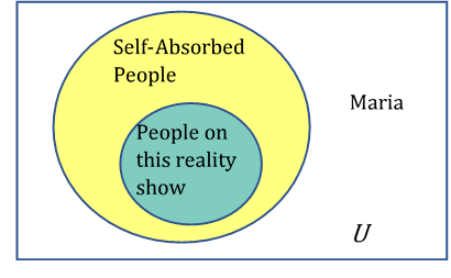
Premise: People on this reality show are self-absorbed.
Premise: Laura is not self-absorbed.
Conclusion: Laura cannot be on this reality show.
This argument is deductive. The argument is valid because Laura is outside of the set of self-absorbed people, so she must also be outside of this set of people on this reality show. Determining if this conclusion is sound is more difficult because determining if someone is self-absorbed is subjective.

1.8.5.17.

Solution.
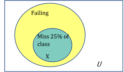
This argument is valid, and it is sound. Because Ethan is in the set of folks who missed 25% of the classes he also falls into the set of failing.

1.8.5.19.

Solution.
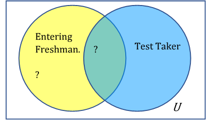
This argument is not valid, and is not sound. We cannot determine if Juan took the test.

1.9 Logical Fallacies
1.9.9 Exercises

2 Financial Math
2.1 Introduction to Spreadsheets
2.1.6 Exercises

2.1.6.13.

Solution.
  1. =1000*103%*103% which gives $1060.90
  2. =1000*(103%)^2 gives the same result of $1060.90, because raising 103% to the second power means the same as multiplying 103% by itself two times.
  3. =1000*(103%)^15 which gives $1557.97 rounded to the nearest cent
  4. Refer to the table at the bottom for part d and part e.
    Note the entry in cell B3 here is = B2*103% and the remaining cells are computed using the fill down feature.
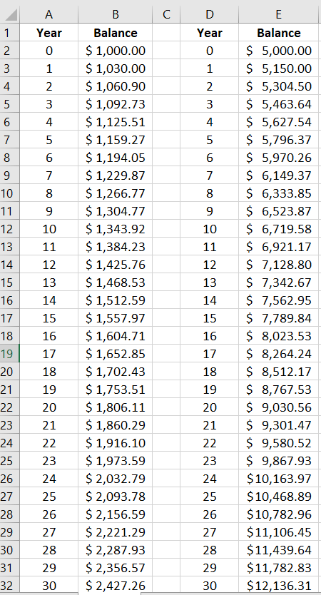
    You will have to wait a minimum of 24 full years, in each case, in order for the balance to finally exceed twice the opening deposit amount.
  5. Since \((103\%)^{23} \lt 2 \lt (103\%)^{24}\text{,}\) the minimum number of full years until the opening deposit doubles must be the same here, for any positive opening balance that we may choose for this account.
A portion of a spreadsheet is shown, which includes cells A1 through E32, and with a title heading of Table 3. Cell A1 shows a column title of Year, and cells A2 through A32 contain values of 0 through 30, respectively. Cells D1 through D32 are a copy of cells A1 through A32. Cell B1 shows a column title of Balance. Cell B2 shows $1,000.00, which corresponds to Year 0 displaying in adjacent cell A1. Cell B3 shows $1,030.00, which is 103% of the $1,000 shown in cell B2. Cell B4 shows $1,060.90, which is 103% of the $1,030.00 shown in cell B3. This pattern continues until we get to cell B32, which shows $2,427.26, and which is 103% of the $2,356.57 amount shown in cell B31. Cell E1 shows a column title of Balance. Cell B2 shows $5,000.00, which corresponds to Year 0 displaying in adjacent cell D1. Cell E3 shows $5,150.00, which is 103% of the $5,000 shown in cell E2. Cell E4 shows $5,304.50, which is 103% of the $5,150.00 shown in cell E3. This pattern continues until we get to cell E32, which shows $12,136.31, and which is 103% of the $11,782.83 amount shown in cell E31.

2.2 Simple and Compound Interest
2.2.11 Exercises

2.2.11.5.

Solution.
  1. \begin{align*} A\amp=20000+20000(0.05)(10)\\ \amp=\$30{,}000 \end{align*}
  2. \begin{align*} A\amp=20000(1+0.05)^{10}\\ \amp=\$32{,}577.89 \end{align*}
The simple interest account would be worth $30,000 and the account that was compounding would be worth $32,577.89 in ten years.

2.2.11.7.

Solution.
\begin{align*} A\amp=1000\left(1+\frac{0.07}{52}\right)^{52*20}\\ \amp\approx \$4{,}051.38 \end{align*}
The account balance is $4,051.38 in 20 years.
Or,
=FV(0.07/52,52*20,0,1000)

2.2.11.9.

Solution.
  1. \begin{align*} A\amp=300\left(1+\frac{0.05}{1}\right)^{1*10}\\ \amp\approx \$488.67 \end{align*}
    There will be $488.67 in the account in 10 years.
    Or,
    =FV(0.05/1,1*10,0,300)
  2. \begin{align*} I\amp=488.67-300\\ \amp=\$188.67 \end{align*}
    $188.67 of the balance will be interest.
  3. \begin{gather*} \frac{188.67}{488.67} \approx 0.3861 \text{ or } 38.61\% \end{gather*}
    The interest makes up 38.61% of the balance.

2.2.11.11.

Solution.
  1. \begin{align*} A\amp=10000\left(1+\frac{0.04}{52}\right)^{52*25}\\ \amp\approx \$27{,}172.37 \end{align*}
    The balance is $27,172.37.
    Or,
    =FV(0.04/52,52*25,0,10000)
  2. \begin{align*} I\amp=27{,}172.37-10{,}000\\ \amp=\$17{,}172.37 \end{align*}
    The interest is $17,172.37.
  3. \begin{gather*} \frac{17{,}172.37}{27{,}172.37} \approx 0.632 \rightarrow 63.2\% \end{gather*}
    The percent that is interest is 63.2%.
  4. \begin{gather*} \frac{10{,}000}{27{,}172.37} \approx 0.368 \rightarrow 36.8\% \end{gather*}
    The percentage that is the principal is 36.2%.

2.2.11.13.

Solution.
\begin{align*} P\amp=\frac{20000}{\left(1+\frac{0.05}{4}\right)^{4*4}}\\ \amp\approx \$16{,}394.79 \end{align*}
The principal required would be $16,394.79
Or,
=PV(0.05/4,4*4,0,20000)

2.2.11.15.

Solution.
  1. Bill =EFFECT(0.0375,12) \(=3.82\%\) and Ted =EFFECT(0.038,1) =3.8%. Bill has an effective rate of 3.82% and Ted has a rate of 3.8%.
  2. \begin{align*} A\amp=6700\left(1+\frac{0.0375}{12}\right)^{12*5}\\ \amp\approx \$8{,}079.38 \end{align*}
    Or, =FV(0.0375/12,5*12,0,6700)
    \begin{align*} A\amp=6500\left(1+\frac{0.038}{1}\right)^{1*5}\\ \amp\approx \$7{,}832.49 \end{align*}
    Or, =FV(0.038,5,0,6500)
    The account balances are $8,079.38 and $7,832.49. So, Bill’s balance is higher.

2.2.11.19.

Solution.
  1. \begin{align*} A\amp= 5000e^{0.045*5}\\ \amp\approx \$6{,}261.61 \end{align*}
    Or, =5000*EXP(0.045*5)
    The account balance is $6,261.61.
  2. \begin{align*} I \amp= 6{,}261.61-5{,}000\\ \amp= \$1{,}261.61 \end{align*}
    The interest earned is $1,261.61
  3. \begin{gather*} \frac{1{,}261.61}{6{,}261.61} \approx 0.2015 \rightarrow 20.15\% \end{gather*}
    The interest is 20.15% of the balance.

2.3 Savings Plans
2.3.5 Exercises

2.3.5.3.

Solution.
  1. \(\frac{750\left(1+\frac{0.0775}{4})^{4*30}-1\right)}{\left(frac{0.0775}{4}\right)}\)
    Or, =FV(0.0775/4,4*30,750)
    In 30 years you will have $348,456.10 in your retirement plan.
  2. \(348{,}456.1 – 4*30*750\text{.}\) You will have earned $258,456.10 in interest.
  3. \(258{,}456.1 /348{,}456.1\text{.}\) The final balance will be about 74.2% interest.

2.3.5.5.

Solution.
  1. In 5 years: \(\frac{130\left(\left(1+\frac{0.09}{12}\right)^{12*5}-1\right)}{\left(\frac{0.09}{12}\right)}\)
    Or, =FV(0.09/12,12*5,130)
    In 25 more years: \(9805.14(1+\frac{0.09}{12})^{12*25}\)
    =FV(0.09/12,12*25,0,9805.14)
    Your final balance will be $92,250.82.
  2. \(92{,}250.82 – 130*5*12\text{.}\) You will earn $84,450.82 in interest.
  3. \(84{,}450.82/92{,}250.82\text{.}\) The final balance will be about 91.5% interest.

2.3.5.7.

Solution.
\(\frac{3500\left(\frac{0.038}{12}\right)}{\left(1+\frac{0.038}{12}\right)^{30}-1}\)
=PMT(0.038/12,30,0,3500)
You should deposit $111.40 each month.

2.3.5.9.

Solution.
\(\frac{450000\left(\frac{0.06}{12}\right)}{\left(1+\frac{0.06}{12}\right)^{12*30}-1}\)
Or, =PMT(0.06/12,12*30,0,450000)
Jamie needs to deposit $447.98 each month.

2.3.5.11.

Solution.
  1. Jose: \(55000\left(1+\frac{0.056}{12}\right)^{12*25}\)
    Or, =FV(0.056/12,12*25,0,55000)
    Jose’s partner:\(\frac{375\left(\left(1+\frac{0.056}{12}\right)^{12*25}-1\right)}{\left(\frac{0.056}{12}\right)}\)
    Or, =FV(0.056/12,12*25,375)
    Jose will have $222,310.85 and his partner will have $244,447.68.
  2. Jose: \(222{,}310.85 – 55{,}000\)
    Jose’s partner: \(24{,}4447.68 – 375*12*25\)
    Jose will earn $167,310.85 and his partner will earn $131,947.68 in interest.
  3. Jose: \(167{,}310.85/222{,}310.85\)
    Jose’s partner: \(13{,}1947.68/244{,}447.68\)
    Jose’s final balance will be about 75.3% interest and Jose’s partner’s final balance will be about 54.0% interest.

2.3.5.13.

Solution.
  1. \(1000\left(1+\frac{0.045}{12}\right)^{12*10}+\frac{100\left(\left(1+\frac{0.045}{12}\right)^{12*10}-1\right)}{\frac{0.045}{12}}\)
    Or, =FV(0.045/12,12*10,100,1000)
    Sylvin will have a final balance of $16,686.80.
  2. \(16{,}686.8 – (1000 + 100*12*10)\text{.}\) Sylvin will earn $3,686.80 in interest.
  3. \(3{,}686.8/16{,}686.8\text{.}\) The final balance will be about 22.1% interest.

2.3.5.15.

Solution.
  1. \(\frac{100\left(\left(1+\frac{0.04}{12}\right)^{12*25}-1\right)}{\frac{0.04}{12}}\)
    Or, =FV(0.04/12,12*25,100)
    Vanessa will have $51,412.95 when she turns 65.
  2. \(\frac{100\left(\left(1+\frac{0.04}{12}\right)^{12*40}-1\right)}{\frac{0.04}{12}}\)
    =FV(0.04/12,12*40,100
    Vanessa would have $118,196.13 if she had started saving when she was 25.

2.4 Loan Payments
2.4.9 Exercises

2.4.9.1.

Solution.
  1. \(P = \frac{700\left(1-\left(1+\frac{5.5\%}{12}\right)^{-12\times 30}\right)}{\frac{5.5\%}{12}}\text{,}\) which gives \(P \approx \$123{,}285.23\)
    or =PV(0.055/12,12*30,-700) [Note 700 is entered as negative, to signify a payment]
  2. \(700 * 12 * 30\) dollars, or $252,000.00 in total payments to the loan company
  3. Interest will be the difference between the total payments, and the amount borrowed. So the interest on this loan is \(\$252{,}000.00 - \$123{,}285.23 = \$128{,}714.77\text{.}\)

2.4.9.3.

Solution.
\(d = \frac{25000\left(\frac{2\%}{12}\right)}{\left(1-\left(1+\frac{2\%}{12}\right)^{-12 \times 4}\right)}\text{,}\) which gives \(d \approx \$542.38\)
or =PMT(0.02/12,48,25000)

2.4.9.5.

Solution.
  1. The loan amount will be 90% of $200,000.00
    \begin{gather*} = (0.9 * \$200{,}000.00)\\ = \$180{,}000.00 \end{gather*}
  2. \(d = \frac{180000\left(\frac{5\%}{12}\right)}{\left(1-\left(1+\frac{5\%}{12}\right)^{-12 \times 30}\right)}\text{,}\) which gives \(d \approx \$966.28\)
    or =PMT(0.05/12,12*30,180000)
  3. \(d = \frac{180000\left(\frac{6\%}{12}\right)}{\left(1-\left(1+\frac{6\%}{12}\right)^{-12 \times 30}\right)}\text{,}\) which gives \(d \approx \$1{,}079.19\)
    or =PMT(0.06/12,12*30,180000)

2.4.9.7.

Solution.
First, we need to find out the amount of the monthly payments for this loan.
\(d = \frac{24000\left(\frac{3\%}{12}\right)}{\left(1-\left(1+\frac{3\%}{12}\right)^{-12 \times 5}\right)}\text{,}\) which gives \(d \approx \$431.25\)
or =PMT(0.03/12,12*5,24000)
The amount still owed three years later, is the present value of the two years of remaining payments on the loan.
\(P = \frac{\left(1-\left(1+\frac{3\%}{12}\right)^{-12 \times 2}\right)}{\frac{3\%}{12}}\text{,}\) which gives \(P \approx \$10{,}033.45\)
or =PV(0.03/12,12*2,-431.25)

2.4.9.11.

Solution.
  1. =PMT(0.05,10,100000,0) which gives $12,950.46.
  2. The total payments will be $129,504.60.
    The interest is the amount over the $100,000 initial investment, or $29,504.60.
    The percentage of the total payment sum representing interest will be \(100(29,504.60/129,504.60)\%\text{,}\) or approximately 22.7827%.

2.4.9.13.

Solution.
  1. =PMT(0.045/12,12*30,250000) which gives $1,266.71.
  2. This will be the present value of the remaining 240 loan payments:
    =PV(0.045/12,12*20,1266.71) which gives $200,223.07.
  3. This will be the present value of the remaining 120 loan payments:
    =PV(0.045/12,12*10,1266.71) which gives $122,223.99.
  4. At the beginning of the repayment period, most of each payment goes to interest (thus the loan balance reduces very slowly at first). Over time, more of each payment shifts to principal, and less to interest. At the end of the loan repayment period, nearly all the payment is going to principal.

2.4.9.17.

Solution.
=PV(0.028/12,4*12,100,0) = $4,535.96. Miao can finance $4,535.96 in equipment to have a monthly loan payment of $100 for 4 years.

2.4.9.21.

Solution.
For the first plan: =FV(0.048/12,20*12,150,0) = $60,251.26. Zahid would have $60,251.26 if he puts in $150 per month for 20 years.
For the second plan: =FV(0.048/12,10*12,300,0) = $46,089.59. Zahid would only have $46,089.59 if he waited and put in $300 per month for 10 years.

2.5 Income Taxes
2.5.14 Exercises

2.5.14.1.

Solution.
A credit decreases your bill more. It decreases your bill by the full amount of the credit. A deduction only decreases your tax bill by a percentage.

2.5.14.5.

Solution.
Yes, you can make adjustments and take a deduction. Adjustments to your income happen before deductions.

2.5.14.7.

Solution.
Shaysiah should itemize because itemizing reduces her taxable income by $15,400. The standard deduction would have reduced her taxable income by $14,600.

2.5.14.9.

Solution.
No, Fredrick should not be concerned. Only the $1000 will be taxed at 22%. The rest of his income will be taxed at a lower level.

2.5.14.13.

Solution.
$16,589 in taxes minus $13,456 for withholdings, and they can claim and $2,500 in credits. This leaves them owing $633.

2.5.14.15.

Solution.
  1. Take the income minus the adjustments \(135000-5600=\$129{,}400\text{.}\) Their adjusted gross income is $129,400.
  2. They should take the standard deduction because itemizing saves them less.
  3. Taxable income: \(129400-29200=100200\)
    Taxes owed: \(10852+0.22*(100200-94300)=\$12{,}150\)
    They owe $12,150 in taxes.
  4. \(12150-15000=-\$2{,}850\) Take the taxes owed minus credits and withholdings. They will receive a refund for $2,850.

2.5.14.17.

Solution.
  1. Gross Income: \(96000+850 = \$96{,}850\)
  2. Adjusted Gross Income: \(96850-26000 = \$70{,}850\)
  3. She should take itemized deductions since they are greater than the standard deduction for head of household.
  4. Taxable Income: \(70850-22600 = \$48{,}250 \)
  5. Tax from Table: \(1655 + 0.12*(48250 - 16550) = \$5{,}459\text{.}\) Owed/Refund: \(5459 – 4000 – 5300 = - \$3{,}841\)
    Janice will receive a refund of $3,841.

2.6 Chapter 2 Review

2.6.1.

Solution.
  1. \(I=1525(0.056)(14)\)
    \(A=1525+1525(0.056)(14)\)
    The interest is $1,195.6 and balance is $2,720.6.
  2. \(A=1525(1+\frac{0.056}{4})^{4\cdot14}\)
    Or, =FV(0.056/4, 4*14, 0, 1525)
    The interest is $1,796.97 and the balance is $3,321.97.
  3. \(A=1525(1+\frac{0.056}{52})^{52\cdot14}\)
    Or, =FV(0.056/52, 52*14, 0, 1525)
    The interest is $1,813.67 and the balance is $3,338.67.
  4. \(A=1525e^{0.056\cdot14}\)
    Or, =1525*EXP(0.056*14)
    The interest is $1,815.08 and the balance is $3,340.08.

2.6.7.

Solution.
  1. \(A= \frac{350((1+\frac{0.065}{12})^{12\cdot25}-1)}{\frac{0.065}{12}}\)
    Or, =FV(0.065/12, 12*25, 350, 0)
    The future value is $262,092.78 and the interest earned is $157,092.78.
  2. \(A= \frac{500((1+\frac{0.065}{4})^{4\cdot15}-1)}{\frac{0.065}{4}}\)
    Or, =FV(0.065/4, 4*15, 500, 0)
    The future value is $50,168.34 and the interest earned is $20,168.34.
  3. \(A= \frac{75((1+\frac{0.045}{52})^{52\cdot30}-1)}{\frac{0.045}{52}}\)
    Or, =FV(0.045/52, 52*30, 75, 0)
    The future value is $247,448.43 and the interest earned is $130,448.43.

3 Statistics
3.1 Overview of the Statistical Process
3.1.22 Exercises

3.1.22.1.

Solution.
A sample is a sub group of the population. A population is the entire group of subjects.

3.1.22.27.

Solution.
Play Barry Manilow to half the crop and don’t play any music to the other half of the crop.

3.2 Describing Data
3.2.24 Exercises

3.2.24.19.

Solution.
The graph would be more effective at displaying the true differences between the categories if the vertical scale started at 0. The vertical axis is missing a label and units, so we can’t tell if those are frequencies or relative frequencies. A flat bar graph (instead of the 3d graph) would be easier to read.

3.2.24.21.

Solution.
This is a poor graph because the vertical axis does not have a numerical scale, so we cannot know how many have each drink as a favorite drink. We also don’t know if the bottom vertical line represents 0, which is potentially misleading.

3.2.24.25.

Solution.
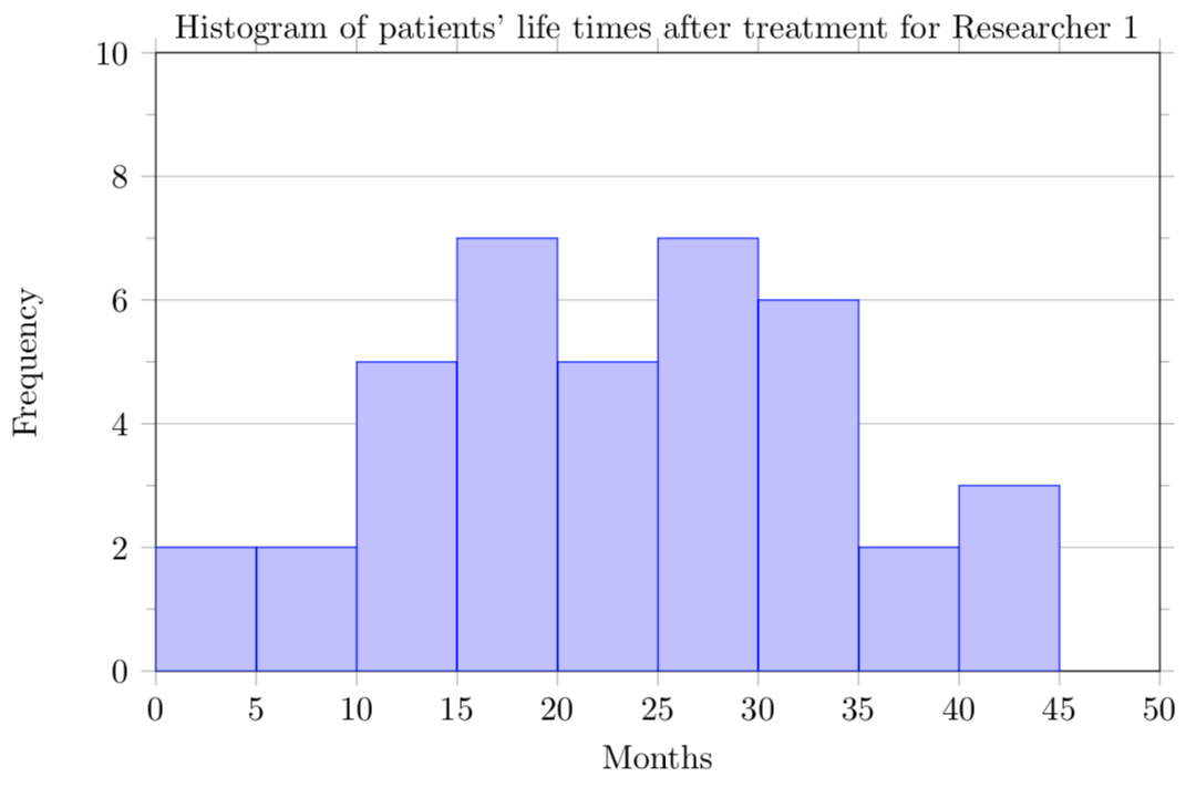
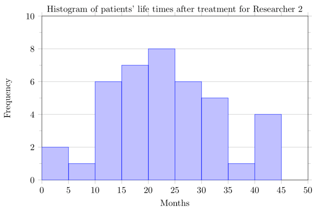
  1. The data for patients of both researchers are symmetric. Researcher’s 1 patients’ data appears to be unimodal, but Researcher 2’s patients’ data may be bimodal or multimodal. The data for Researcher 1’s patients does not have any outliers, but the data for Researcher’s 2 may have outliers between 0 and 5 months or 40 and 45 months.

3.3 Summary Statistics: Measures of Center
3.3.7 Exercises

3.3.7.1.

Solution.
  1. In Excel:
    =average(7.50,25,10,10,7.50,8.25,9,5,15,8,7.25,7.50,8,7,12)
    \(=\$9.80\)
    There are 15 amounts shown, so \(n=15\text{.}\) The mean is:
    \begin{align*} \bar{x} \amp= \frac{(7.50+25+10+10+7.50+8.25+9+5+15+8+7.25+7.50+8+7+12)}{15}\\ \amp=\$9.80 \end{align*}
  2. In Excel:
    =median(7.50,25,10,10,7.50,8.25,9,5,15,8,7.25,7.50,8,7,12)
    \(=\$8.00\)
    There are 15 times shown, so \(n=15\text{.}\) We start by listing the data in order:
    $5, $7, $7.25, $7.50, $7.50, $7.50, $8, $8, $8.25, $9, $10, $10, $12, $15, $25
    \(Median=\$8.00\)
  3. Since the mean is greater than the median, we would expect the distribution will be skewed right.

3.3.7.3.

Solution.
  1. In Excel:
    =average(15.2,18.8,19.3,19.7,20.2,21.8,22.1,29.4)
    \(=20.81\) seconds
    There are 8 times shown, so \(n=8\text{.}\)
    \begin{align*} \bar{x} \amp= \frac{(15.2+18.8+19.3+19.7+20.2+21.8+22.1+29.4)}{15}\\ \amp=20.81 \text{ seconds} \end{align*}
  2. In Excel:
    =median(15.2,18.8,19.3,19.7,20.2,21.8,22.1,29.4)
    \(=19.95\) seconds
    There are 8 times shown, so \(n=8\text{.}\) The times are given already in order:
    15.2, 18.8, 19.3, 19.7, 20.2, 21.8, 22.1, 29.4
    \begin{align*} Median\amp=\frac{19.7+20.2}{2}\\ \amp=19.95 \text{ seconds} \end{align*}
  3. Since the mean and median are approximately equal, we would expect that the distribution is symmetric.

3.3.7.5.

Solution.
  1. In GeoGebra Classic, enter the costs into the column A and frequencies into column B of the spreadsheet and use the β€œOne Variable Analysis” function. Then use the β€œShow Statistics” option.
    \begin{gather*} Mean=33.8 \text{ thousand dollars} \end{gather*}
    The sum of the frequencies is 75, so \(n=75\)
    \begin{align*} \bar{x}\amp=\frac{15\cdot 3+20\cdot 7+25\cdot 10+30\cdot 15+35\cdot 13+40\cdot 11+45\cdot 9+50\cdot 7}{75}\\ \amp=33.8 \text{ thousand dollars} \end{align*}
  2. In GeoGebra Classic, enter the costs into the column A and frequencies into column B of the spreadsheet and use the β€œOne Variable Analysis” function. Then use the β€œShow Statistics” option.
    \begin{gather*} Median=35 \text{ thousand dollars} \end{gather*}
    Since there are 75 values (an odd number), we know that the median will be the single middle data value. Because \(\frac{75}{2}=37.5\text{,}\) we know it will be the 38th value in the list. The 38th value is 35, so the median is 35 thousand dollars.
  3. Since the mean is less than the median, we would expect the distribution to be skewed left.

3.3.7.7.

Solution.
  1. For Researcher 1:
    In Excel:
    =average(A1:A40)
    \(=23.6\) months.
    =median(A1:A40)
    \(=24\) months
    The mean for Researcher 1’s patients is 23.6 months, and the median for Researcher’s 1 patients is 24 months.
    For Researcher 2:
    In Excel:
    =average(A1:A40)
    \(=22.8\) months
    =median(A1:A40)
    \(=22\) months
    The mean for Researcher 2’s patients is 22.8 months, and the median is 22 months
  2. Both the mean and median for Researcher 1’s patients are greater than the mean and median for Researcher 2’s patients. So, on average, Researcher 1’s patients have a longer life time after starting the cancer treatment than Researcher 2’s patients.

3.3.7.9.

Solution.
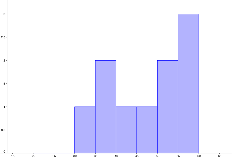
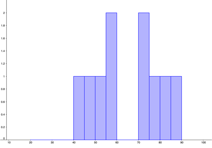
GeoGebra was used to create the histograms. You should check with your instructor to see if histograms are to be hand-drawn or computer generated. Answers will vary depending on the size of the margins and the programs you are using.
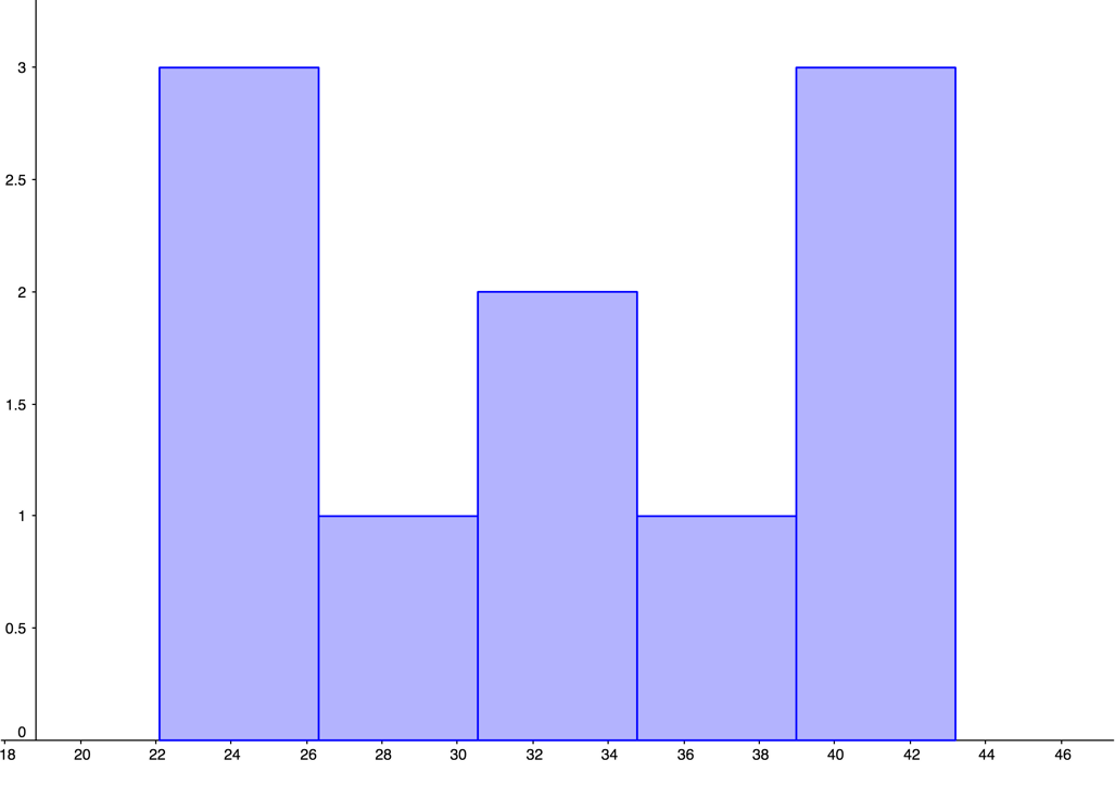
  1. Figure 3.3.16. Histogram for Average Number of Pieces Correctly Remembered by Non-players
    Figure 3.3.17. Histogram for Average Number of Pieces Correctly Remembered by Beginners
    Figure 3.3.18. Histogram for Average Number of Pieces Correctly Remembered by Tournament Players
  2. The mean number of pieces correctly remembered for non-players was 33.65 pieces.
    The mean number of pieces correctly remembered for beginners was 47.6 pieces.
    The mean number of pieces correctly remembered for tournament players was 64.98 pieces.
  3. The median number of pieces correctly remembered for non-players was 33.5 pieces.
    The median number of pieces correctly remembered for beginners was 51.3 pieces.
    The median number of pieces correctly remembered for tournament players was 71.1 pieces.
  4. The distribution for non-players appears to be uniform. The distribution for beginners looks unimodal and left-skewed. The distribution for tournament players appears bimodal and symmetric.
    The mean and median number of pieces correctly remembered were both greatest for tournament players, with non-players having the smallest mean and median of pieces correctly remembered.

3.3.7.11.

Solution.
  1. There are many possible answers for this problem. Three data sets with 5 values each that have the same mean but different medians are:
    0, 0, 0, 0, 10
    0, 0, 2, 4, 4
    0, 1, 1, 1, 7
  2. There are many possible answers for this problem. Three data sets with 5 values that have the same median but different means are:
    10, 10, 10, 10, 10
    0, 0, 10, 15, 20
    1, 5, 10, 10, 10

3.3.7.15.

Solution.
  1. Incomes are skewed to the right so the mean would be greater than the median.
  2. Weights are approximately symmetric so the mean would be about the same as the median.
  3. Number of children is skewed to the right so the mean would be greater than the median.
  4. Medical costs for all adults are most likely skewed to the right so the mean would be greater than the median.
  5. Medical costs for adults 65+ may be symmetric or skewed to the right. Answer according to the shape you chose.

3.4 Summary Statistics: Measures of Variation
3.4.10 Exercises

3.4.10.1.

Solution.
  1. In Excel:
    Entering the data values into cells A1 through A15.
    \begin{align*} s\amp=stdev.s(A1:A15)\\ \amp=\$4.82 \end{align*}
    From ExerciseΒ 3.3.7.1, the mean is $9.80. There are 15 data values, so \(n=15\text{.}\)
    We will make a table of data values, their deviations from the mean, and the squared deviations:
    Data Value Deviation Deviation Squared
    \(7.5\) \(7.5-9.8=-2.3\) \((-2.3)^2=5.29\)
    \(25\) \(25-9.8=15.2\) \((15.2)^2=231.04\)
    \(10\) \(10-9.8=0.2\) \((0.2)^2=0.04\)
    \(10\) \(10-9.8=0.2\) \((0.2)^2=0.04\)
    \(7.5\) \(7.5-9.8=-2.3\) \((-2.3)^2=5.29\)
    \(8.25\) \(8.25-9.8=-1.55\) \((-1.55)^2=2.4\)
    \(9\) \(9-9.8=-0.8\) \((-0.8)^2=0.64\)
    \(5\) \(5-9.8=-4.8\) \((-4.8)^2=23.04\)
    \(15\) \(15-9.8=5.2\) \((5.2)^2=27.04\)
    \(8\) \(8-9.8=-1.8\) \((-1.8)^2=3.24\)
    \(7.25\) \(7.25-9.8=-2.55\) \((-2.55)^2=6.5\)
    \(7.5\) \(7.5-9.8=-2.3\) \((-2.3)^2=5.29\)
    \(8\) \(8-9.8=-1.8\) \((-1.8)^2=3.24\)
    \(7\) \(7-9.8=-2.8\) \((-2.8)^2=7.84\)
    \(12\) \(12-9.8=2.2\) \((2.2)^2=4.84\)
    Next, we add the squared deviations and get \(5.29 + 231.04 + 0.04 + 0.04 + 5.29 + 2.4 + 0.64 + 23.04 + 27.04 + 3.24 + 6.5 + 5.29 + 3.24 + 7.84 + 4.84 = 325.78\) dollars-squared.
    The sample standard deviation is:
    \begin{align*} s\amp=\sqrt{\frac{325.78}{14}}\\ \amp=\$4.82 \end{align*}
  2. In GeoGebra:
    In GeoGebra Classic, enter the data values into the column A of the spreadsheet and use the β€œOne Variable Analysis” function. Then use the β€œShow Statistics” option to find the five-number summary.
    Min Q1 Median Q3 Max
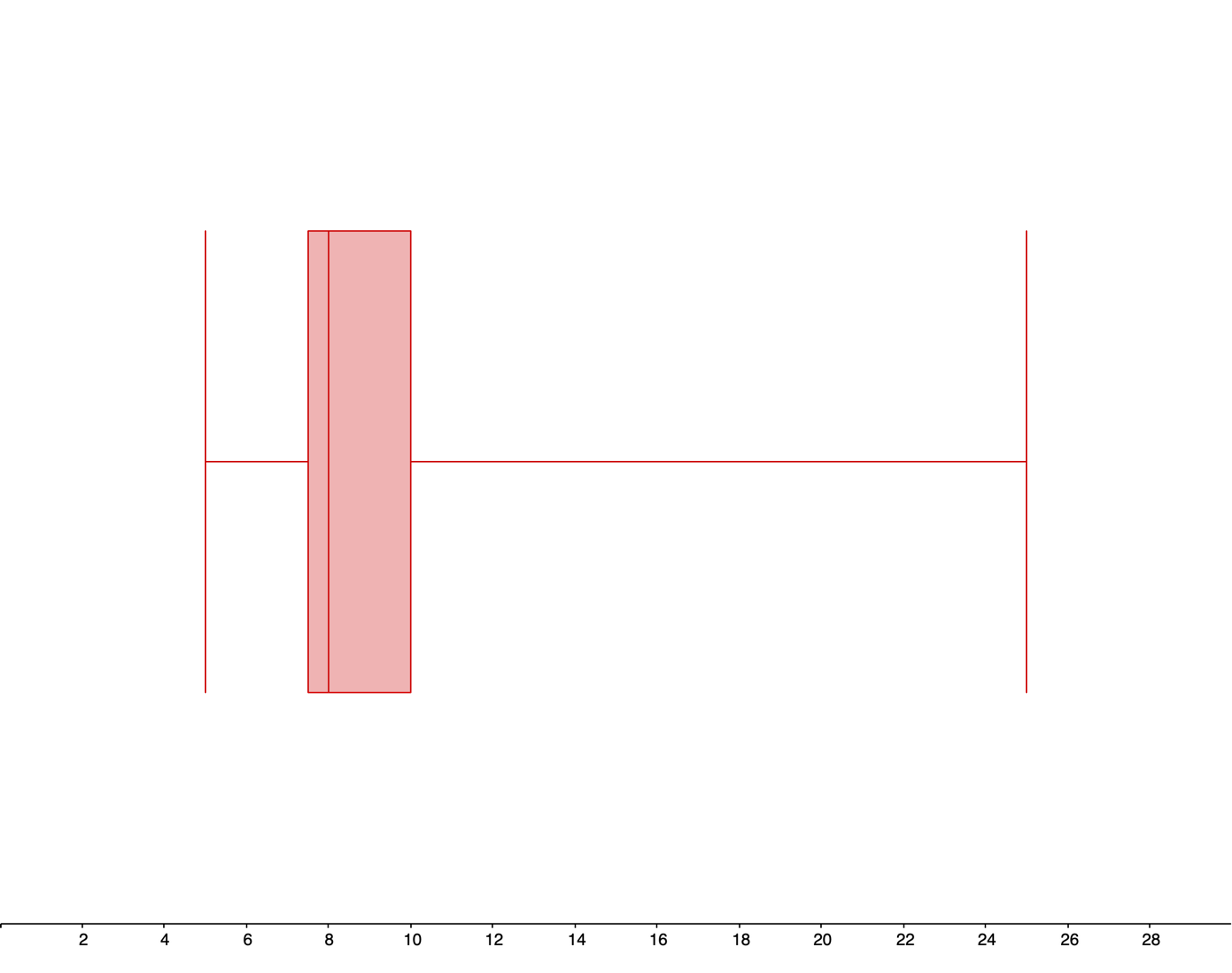
    $5 $7.50 $8 $10 $25
    From ExerciseΒ 3.3.7.1, the data listed in order is:
    $5.00, $7.00, $7.25, $7.50, $7.50, $7.50, $8.00, $8.00, $8.25, $9.00, $10.00, $10.00, $12.00, $15.00, $25.00
    Also from ExerciseΒ 3.3.7.1, there are 15 data values (\(n=15\)), and the median is $8.00. The lower half of the data is:
    $5.00, $7.00, $7.25, $7.50, $7.50, $7.50, $8.00
    The median of the lower half is $7.50, so the lower quartile \(Q_{1}\) is $7.50.
    The upper half of the data is:
    $8.25, $9.00, $10.00, $10.00, $12.00, $15.00, $25.00
    The median of the upper half is $10.00, so the upper quartile \(Q_{3}\) is $10.00.
    The smallest and largest data values are $5.00 and 25.00, respectively, so the min and max are $5.00 and $25.00. The five-number summary is:
    Min Q1 Median Q3 Max
    $5 $7.50 $8 $10 $25
  3. The range is:
    \begin{align*} Range \amp= Max - Min\\ \amp=25-5\\ \amp=\$20 \end{align*}
    The interquartile range (IQR) is:
    \begin{align*} IQR \amp= Q_{3} - Q_{1}\\ \amp=10-7.5\\ \amp=\$2.50 \end{align*}

3.4.10.3.

Solution.
  1. In Excel:
    I entered the data values into cells A1 through A9.
    The standard deviation is:
    \begin{align*} s\amp=stdev.s(A1:A9)\\ \amp=4.068 \text{ seconds} \end{align*}
  2. In GeoGebra:
    In GeoGebra Classic, enter the data values into the column A of the spreadsheet and use the β€œOne Variable Analysis” function. Then use the β€œShow Statistics” option to find the five-number summary.
    Min Q1 Median Q3 Max
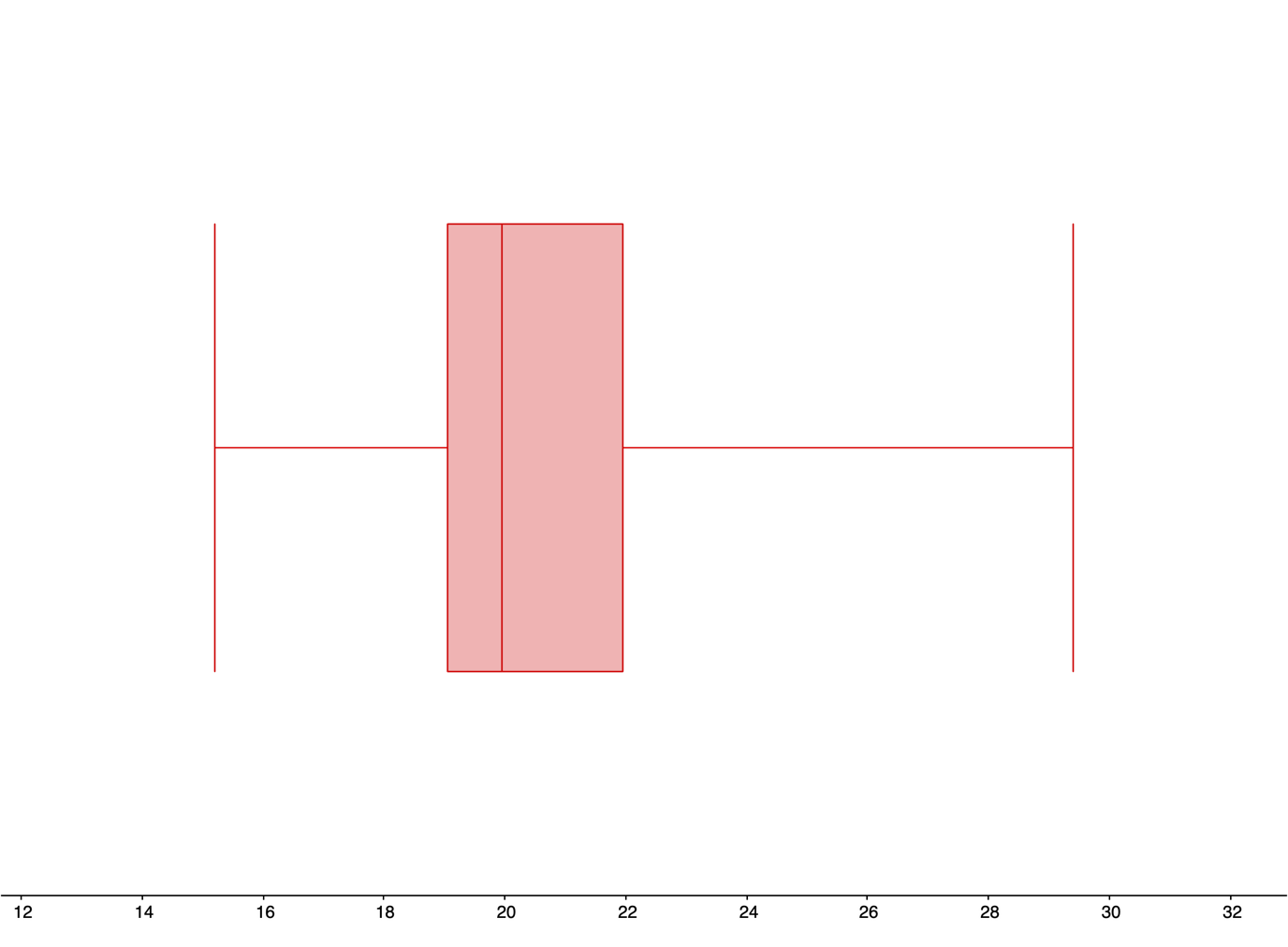
    15.2 seconds 19.05 seconds 19.95 seconds 21.95 seconds 29.4 seconds
  3. The range is:
    \begin{align*} Range \amp= Max - Min\\ \amp=29.4-15.2\\ \amp=14.2 \text{ seconds} \end{align*}
    The interquartile range (IQR) is:
    \begin{align*} IQR \amp= Q_{3} - Q_{1}\\ \amp=21.95-19.05\\ \amp=2.9 \text{ seconds} \end{align*}

3.4.10.5.

Solution.
  1. In GeoGebra:
    In GeoGebra Classic, enter the costs into column A and frequencies into column B of the spreadsheet and use the β€œOne Variable Analysis” function. Then use the β€œShow Statistics” option. The standard deviation is:
    \begin{gather*} s=9.58 \text{ thousand dollars} \end{gather*}
    From ExerciseΒ 3.3.7.5, the mean is 33.8 thousand dollars.
    The mean and the standaed deviation together tell us that, on average, the cars at the local dealership are $9,580 from the mean price of $33,800.
  2. In GeoGebra:
    In GeoGebra Classic, enter the data values into the column A of the spreadsheet and use the β€œOne Variable Analysis” function. Then use the β€œShow Statistics” option to find the five-number summary.
    Min Q1 Median Q3 Max
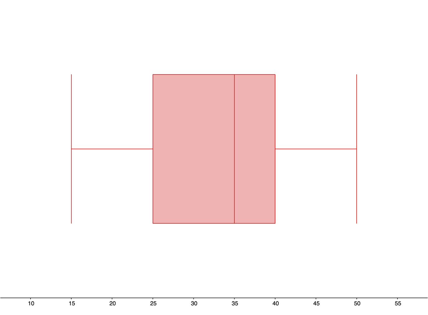
    15 thousand
    dollars
    25 thousand
    dollars
    35 thousand
    dollars
    40 thousand
    dollars
    50 thousand
    dollars
  3. The range is:
    \begin{align*} Range \amp= Max - Min\\ \amp=50-15\\ \amp=35 \text{ thousand dollars} \end{align*}
    The interquartile range (IQR) is:
    \begin{align*} IQR \amp= Q_{3} - Q_{1}\\ \amp=40-15\\ \amp=25 \text{ thousand dollars} \end{align*}

3.4.10.7.

Solution.
  1. In GeoGebra:
    In GeoGebra Classic, enter the data values for Researcher 1 into column A of the spreadsheet, and enter the data values for Researcher 2 into column B of the spreadsheet. Then use the β€œMultiple Variable Analysis” function. Then use the β€œShow Statistics” function to display the sample standard deviation for each set of data values.
    The sample standard deviation for Researcher 1 is 11.25 months. The sample standard deviation for Research 2 is 11.38 months.
  2. In GeoGebra:
    In GeoGebra Classic, enter the data values for Researcher 1 into column A of the spreadsheet, and enter the data values for Researcher 2 into column B of the spreadsheet. Then use the β€œMultiple Variable Analysis” function. Then use the β€œShow Statistics” function to display the sample standard deviation for each set of data values.
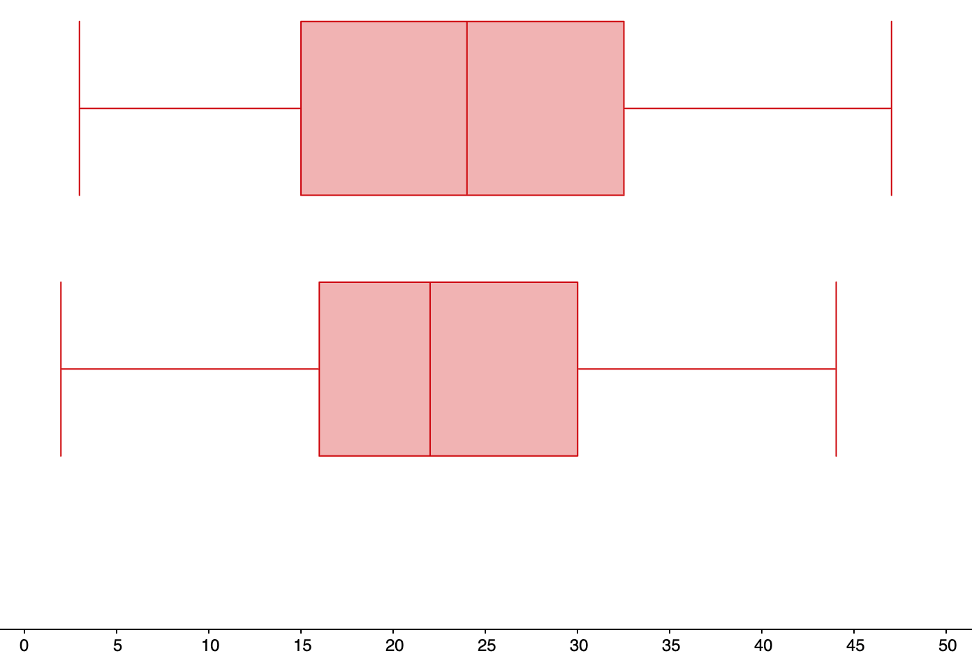
    The 5-number summary for Researcher 1 is:
    Min Q1 Median Q3 Max
    3 months 15 months 24 months 32.5 months 47 months
    The 5-number summary for Researcher 2 is:
    Min Q1 Median Q3 Max
    2 months 16 months 22 months 30 months 44 months
  3. The range for Researcher 1 is:
    \begin{align*} Range \amp= Max - Min\\ \amp=47-3\\ \amp=44 \text{ months} \end{align*}
    The interquartile range (IQR) for researcher 1 is:
    \begin{align*} IQR \amp= Q_{3} - Q_{1}\\ \amp=32.5-15\\ \amp=17.5 \text{ months} \end{align*}
    The range for Researcher 2 is:
    \begin{align*} Range \amp= Max - Min\\ \amp=44-2\\ \amp=42 \text{ months} \end{align*}
    The interquartile range (IQR) for Researcher 2 is:
    \begin{align*} IQR \amp= Q_{3} - Q_{1}\\ \amp=30-16\\ \amp=14 \text{ months} \end{align*}
  4. In GeoGebra Classic, enter the data values for Researcher 1 into column A of the spreadsheet, and enter the data values for Research 2 into column B of the spreadsheet. Then use the β€œMultiple Variable Analysis” function. Then select β€œStacked BoxPlots” from the drop-down menu.
    Researcher 1 has a larger minimum, median, 3rd quartile, and maximum than Researcher 2. For Researcher 1, 50% of the patients live longer than 24 months after treatment, compared to 50% of patients living longer than 22 months after treatment for Researcher 1.
    Researcher 2 has less variation in the life times than Researcher 1, with an IQR of 14 months for Researcher 2, compared to an IQR 16.5 months for Researcher 1.

3.4.10.9.

Solution.
  1. In GeoGebra:
    In GeoGebra Classic, enter the data values for non-players into column A of the spreadsheet, enter the data values for beginners into column B of the spreadsheet, and enter the data value for tournament players into column C of the spreadsheet. Then use the β€œMultiple Variable Analysis” function. Then use the β€œShow Statistics” function to display the sample standard deviation for each set of data values.
    The sample standard deviation for non-players is 8.033 chess pieces. The sample standard deviation for beginners is 9.031 chess pieces. The sample standard deviation for tournament players is 15.622 chess pieces.
  2. In GeoGebra:
    In GeoGebra Classic, enter the data values for non-players into column A of the spreadsheet, enter the data values for beginners into column B of the spreadsheet, and enter the data value for tournament players into column C of the spreadsheet. Then use the β€œMultiple Variable Analysis” function. Then use the β€œShow Statistics” function to display the sample standard deviation for each set of data values.
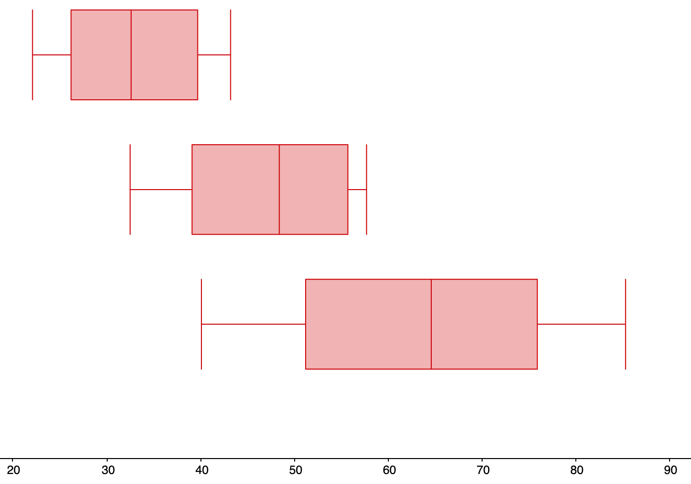
    The 5-number summary for non-players is:
    Min Q1 Median Q3 Max
    22.1 chess
    pieces
    26.2 chess
    pieces
    32.6 chess
    pieces
    39.7 chess
    pieces
    43.2 chess
    pieces
    The 5-number summary for beginners is:
    Min Q1 Median Q3 Max
    32.5 chess
    pieces
    39.1 chess
    pieces
    48.4 chess
    pieces
    55.7 chess
    pieces
    57.7 chess
    pieces
    The 5-number summary for tournament players is:
    Min Q1 Median Q3 Max
    40.1 chess
    pieces
    51.2 chess
    pieces
    64.6 chess
    pieces
    75.9 chess
    pieces
    85.3 chess
    pieces
  3. The range for non-players is:
    \begin{align*} Range \amp= Max - Min\\ \amp=43.2-22.1\\ \amp=21.2 \text{ chess pieces} \end{align*}
    The interquartile range (IQR) for non-players is:
    \begin{align*} IQR \amp= Q_{3} - Q_{1}\\ \amp=39.7-26.2\\ \amp=13.5 \text{ chess pieces} \end{align*}
    The range for beginners is:
    \begin{align*} Range \amp= Max - Min\\ \amp=57.7-32.5\\ \amp=25.2 \text{ chess pieces} \end{align*}
    The interquartile range (IQR) for beginners is:
    \begin{align*} IQR \amp= Q_{3} - Q_{1}\\ \amp=55.7-39.1\\ \amp=16.6 \text{ chess pieces} \end{align*}
    The range tournament players for is:
    \begin{align*} Range \amp= Max - Min\\ \amp=85.3-40.1\\ \amp=45.2 \text{ chess pieces} \end{align*}
    The interquartile range (IQR) for tournament players is:
    \begin{align*} IQR \amp= Q_{3} - Q_{1}\\ \amp=75.9-51.2\\ \amp=24.7 \text{ chess pieces} \end{align*}
  4. Tournament players did the best at remembering positions (as shown by all of the numbers of their 5-number summary being larger than the corresponding numbers for the other two groups). However, tournaments players were not completely superior to the other two groups; the best non-players remembered more chess pieces than the worst tournament players. Also tournament players had more variation in how much they.

3.4.10.11.

Solution.
  1. There are many possible answers for this question. For example, the data sets {10, 10, 10, 10, 10} and {9, 9, 10, 11, 11} have the same mean of 10 units, but different standard deviations (0 and 1, respectively).
  2. There are many possible answers for this question. For example, the data sets {2, 2, 2, 2, 2} and {9, 9, 9, 9, 9} have the same standard deviation of 0, but different means (2 and 9, respectively).

3.4.10.13.

Solution.
  1. The 25th, 50th, and 75th percentiles are, respectively, the 1st quartile, median, and 3rd quartile for the data sets. Reading the boxplot for CPAs, the 25th, 50th, and 75th percentiles for CPAs’ salaries are, respectively, $40,000, $75,000, and $90,000. Reading the boxplot for actuaries, the 25th, 50th, and 75th percentiles for actuaries’ salaries are, respectively, $75,000, $90,000, and $94,000
  2. Deshawn’s salary (the median salary for an actuary) is $90,000; Kelsey’s salary (the first quartile salary) is also $75,000. So Deshawn makes more than Kelsey, by $15,000.
  3. 75% of actuaries make more than the median salary of a CPA ($75,000).
  4. 25% of all CPAs earn less than all actuaries.

3.4.10.15.

Solution.
  1. \begin{align*} Z\amp=\frac{\text{data value}-\text{mean}}{\text{standard deviation}}\\ \amp=\frac{21.4-25}{1.15}\\ \amp=-3.13 \text{ standard deviations} \end{align*}
  2. The \(Z\)-score for the gas mileage of the car is -3.13 standard deviations.

3.4.10.17.

Solution.
  1. In GeoGebra:
    In GeoGebra Classic, enter the data values into the column A of the spreadsheet and use the β€œOne Variable Analysis” function. Then use the β€œShow Statistics” option to find the mean and standard deviation.
    The mean is 46.2 hours per year, and the standard deviation is 6.16 hours per year.
  2. \begin{align*} Z\amp=\frac{\text{data value}-\text{mean}}{\text{standard deviation}}\\ \amp=\frac{42-46.2}{6.16}\\ \amp=-0.68 \text{ standard deviations} \end{align*}
    The \(Z\)-score for a city with an average delay time of 42 hours per year is -0.68 standard deviations.

3.4.10.19.

Solution.
\begin{align*} Z_{Math}\amp=\frac{\text{data value}-\text{mean}}{\text{standard deviation}}\\ \amp=\frac{89-75}{7}\\ \amp=2 \text{ standard deviations} \end{align*}
\begin{align*} Z_{English}\amp=\frac{\text{data value}-\text{mean}}{\text{standard deviation}}\\ \amp=\frac{65-53}{4}\\ \amp=3 \text{ standard deviations} \end{align*}
Because the \(Z\)-score of my English test is greater than the \(Z\)-score of my math test, I did better on the English test than I did on the math test.

3.4.10.21.

Solution.
\begin{align*} Z_{Poe}\amp=\frac{\text{data value}-\text{mean}}{\text{standard deviation}}\\ \amp=\frac{20.2-16.5}{1.85}\\ \amp=2 \text{ standard deviations} \end{align*}
\begin{align*} Z_{Gibson}\amp=\frac{\text{data value}-\text{mean}}{\text{standard deviation}}\\ \amp=\frac{107-81}{13}\\ \amp=2 \text{ standard deviations} \end{align*}
Because the \(Z\)-scores for the heights of Poe (the Clydesdale horse) and Gibson (the Great Dane) are the same, neither animal is taller than the other when compared to their respective breeds.

3.5 Chapter 3 Review

3.5.3.

Solution.
  1. The population being studied is PCC Students.
  2. Categorical or Qualitative
  3. 23% is a statistic because it is from a sample.
  4. The margin of error is 4%.
  5. \(23\% - 4\% = 19\%\) and \(23\% + 4\% = 27\%\text{.}\) The confidence interval is \((19\%, 27\%)\text{.}\)
  6. We are confident that the true proportion of all PCC students who prefer to study at the library is between 19% and 27%

3.5.11.

Solution.
  1. The mean is $4.78 per gallon. The median is $4.75 per gallon.
  2. The mean and median is about the same value therefore the data is symmetric.
  3. The standard deviation is $1.34 per gallon.
  4. \(z_{\$3.25}=\frac{\$3.25-\$4.78}{\$1.34}=\frac{-\$1.53}{\$1.34}=-1.14\)
    \(z_{\$8.95}=\frac{\$8.95-\$4.78}{\$1.34}=\frac{\$4.17}{\$1.34}=3.11\)
  5. Min Q1 Median Q3 Max
    $3.25 $3.75 $4.75 $5.00 $8.95
  6. \(\text{Range}=\$8.95-\$3.25=\$5.70\)
    \(\text{IQR}=\$5-\$3.75=\$1.25\)
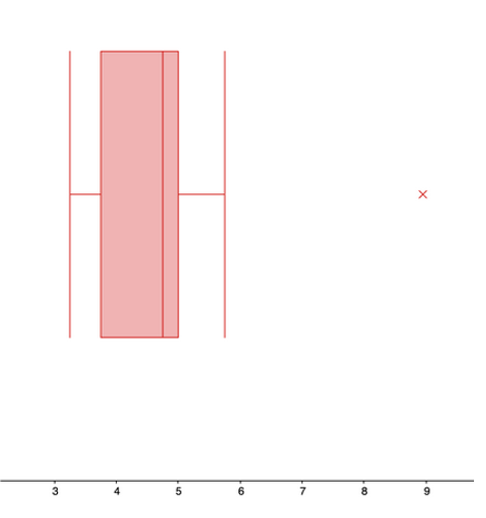
  7. Boxplot using the 5-number summary above showing one outlier at $8.95

3.6 The Normal Distribution
3.6.8 Exercises

3.6.8.7.

Solution.
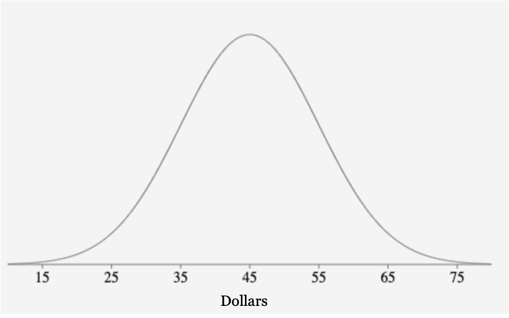
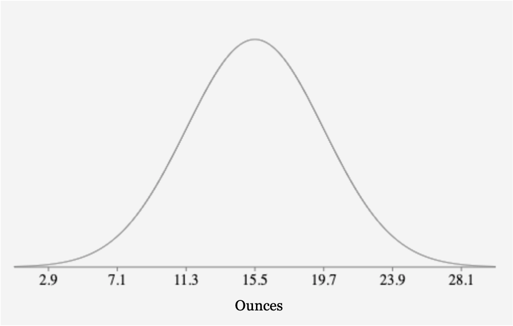
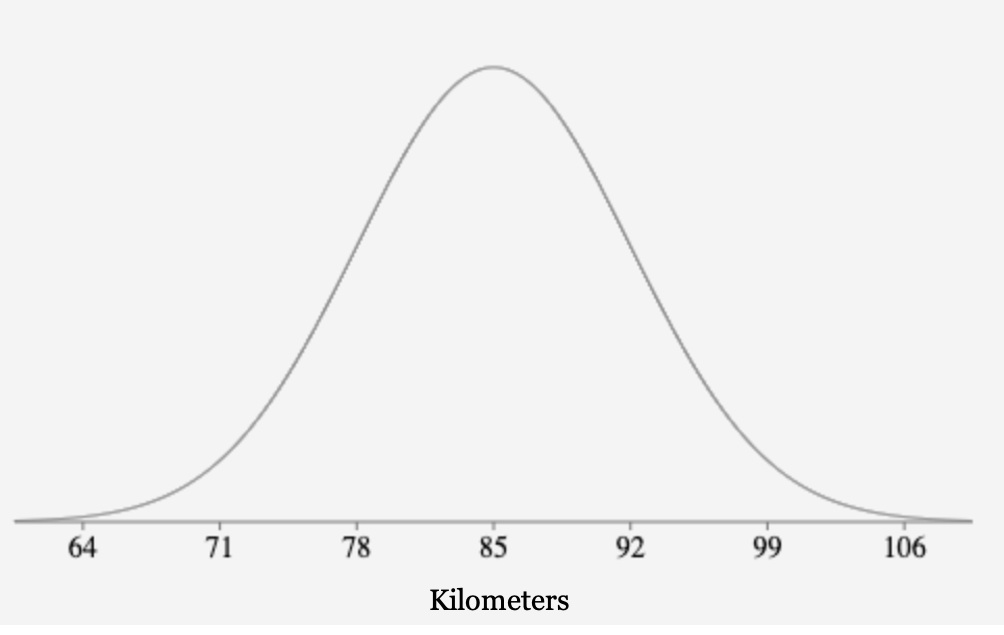
Approximately 99.7% of the values fall within three standard deviations of the mean.

3.6.8.9.

Solution.
Approximately 27% of the values fall between the first and second standard deviations from the mean.

3.6.8.11.

Solution.
Approximately 4.7% of the values fall between the second and third standard deviations from the mean.

3.6.8.13.

Solution.
Approximately 34% of the values fall between the mean and one standard deviation below the mean.

3.6.8.29.

Solution.
The confidence interval is \((\$2.20, \$2.50)\text{.}\) This means that we are 95% confident that the true average amount of change for all those who carry a purse is between $2.20 and $2.50.

3.6.8.31.

Solution.
The margin of error is 0.2156 cm. The confidence interval is approximately \((82.28, 84.72)\text{.}\) This means that we are 95% confident that the true population parameter is between approximately 82.28 and 84.72 cm.

4 Probability
4.1 Contingency Tables
4.1.10 Exercises

4.1.10.1.

Solution.
Food Insecure Not Food Insecure Total
Housing Insecure 380 60 440
Not Housing Insecure 300 460 760
Total 680 520 1200

4.1.10.3.

Solution.
Breakfast No Breakfast Total
Floss 12 49 61
No Floss 3 8 11
Total 15 57 72

4.1.10.7.

Solution.
  1. \begin{align*} \text{P(In morning class)}\amp=\frac{39}{65}\\ \amp= 0.60\text{ or } 60\% \end{align*}
  2. \begin{align*} \text{P(Earned a C)}\amp=\frac{25}{65}\\ \amp\approx 0.385 \text{ or } 38.5\% \end{align*}
  3. \begin{align*} \text{P(Earned an A and in afternoon class)}\amp=\frac{10}{65}\\ \amp\approx 0.154 \text{ or } 15.4\% \end{align*}
  4. \begin{align*} \text{P(Earned an A given in morning class)}\amp=\frac{8}{39}\\ \amp\approx 0.205 \text{ or } 20.5\% \end{align*}
  5. \begin{align*} \text{P(In morning class or earned B)}\amp=\frac{43}{65}\\ \amp\approx 0.662 \text{ or } 66.2\% \end{align*}

4.1.10.9.

Solution.
  1. \begin{align*} \text{P(no credit cards)}\amp=\frac{27}{81}\\ \amp\approx 0.333 \text{ or } 33.3\% \end{align*}
  2. \begin{align*} \text{P(one credit card)}\amp=\frac{15}{81}\\ \amp\approx 0.185 \text{ or } 18.5\% \end{align*}
  3. \begin{align*} \text{P(no credit cards and over age 35)}\amp=\frac{18}{81}\\ \amp\approx 0.222 \text{ or } 22.2\% \end{align*}
  4. \begin{align*} \text{P(between ages of 18 and 35,or have zero credit cards)}\amp=\frac{51}{81}\\ \amp\approx 0.630 \text{ or } 63.0\% \end{align*}
  5. \begin{align*} \text{P(no credit cards given between ages of 18 and 35)}\amp=\frac{9}{33}\\ \amp\approx 0.273 \text{ or } 27.3\% \end{align*}
  6. \begin{align*} \text{P(no credit cards given over age 35)}\amp=\frac{18}{48}\\ \amp=0.375 \text{ or } 37.5\% \end{align*}
  7. Yes, it appears that having no credit cards depends on age. The probability of having no credit cards for people over age 35 is significantly greater than the probability of having no credits for people between the ages of 18 and 35.

4.1.10.11.

Solution.
  1. \begin{align*} \text{P(not survive)}\amp=\frac{1490}{2201}\\ \amp\approx 0.677 \text{ or } 67.7\% \end{align*}
  2. \begin{align*} \text{P(crew)}\amp=\frac{885}{2201}\\ \amp\approx 0.402 \text{ or } 40.2\% \end{align*}
  3. \begin{align*} \text{P(first class and not survive)}\amp=\frac{122}{2201}\\ \amp\approx 0.055 \text{ or } 5.5\% \end{align*}
  4. \begin{align*} \text{P(not survive or crew)}\amp=\frac{1702}{2201}\\ \amp\approx 0.773 \text{ or } 77.3\% \end{align*}
  5. \begin{align*} \text{P(survived given first class)}\amp=\frac{203}{325}\\ \amp\approx 0.625 \text{ or } 62.5\% \end{align*}
  6. \begin{align*} \text{P(survived given second class)}\amp=\frac{118}{285}\\ \amp\approx 0.414 \text{ or } 41.4\% \end{align*}
  7. \begin{align*} \text{P(survived given third class)}\amp=\frac{178}{706}\\ \amp\approx 0.252 \text{ or } 25.2\% \end{align*}
  8. Yes, it does appear that survival depended on the passenger’s class. The probability of survival for first class passengers is significantly greater than the probability of survival for second class passengers and is more than double the probability of survival for third class passengers.

4.1.10.13.

Solution.
  1. Game/Software No Game/Software Total
    Computer 10% 5% 15%
    No Computer 15% 70% 85%
    Total 25% 75% 100%
  2. \begin{align*} \text{P(no computer and no game/software)}\amp=\frac{70\%}{100\%}\\ \amp=0.7 \text{ or } 70\% \end{align*}
  3. \begin{align*} \text{P(computer or game/software)}\amp=\frac{30\%}{100\%}\\ \amp=0.3 \text{ or } 30\% \end{align*}
  4. \begin{align*} \text{P(game/software given computer)}\amp=\frac{10\%}{15\%}\\ \amp\approx 0.667 \text{ or } 66.7\% \end{align*}
  5. \begin{align*} \text{P(game/software given no computer)}\amp=\frac{15\%}{85\%}\\ \amp\approx 0.176 \text{ or } 17.6\% \end{align*}
  6. Purchasing a game/software and purchasing a computer appear to be depended. The probability of purchasing a game/software for computer buyers was almost 50% greater than the probability of purchasing a game/software among customers who did not purchase a computer.

4.1.10.15.

Solution.
  1. Hardcover Paperback Total
    Fiction 13 59 72
    Nonfiction 15 8 23
    Total 28 67 95
  2. \begin{align*} \text{P(non-fiction and paperback)}\amp=\frac{8}{95}\\ \amp\approx 0.084 \text{ or } 8.4\% \end{align*}
  3. \begin{align*} \text{P(fiction given hardcover)}\amp=\frac{13}{28}\\ \amp\approx 0.464 \text{ or } 46.4\% \end{align*}

4.2 Theoretical Probability
4.2.15 Exercises

4.3 Expected Value
4.3.2 Exercises

4.3.2.1.

Solution.
  1. Die roll Gold Silver Black
    Outcome $3 $2 -$1>
    Probability \(3/37\) \(6/37\) \(28/37\)
  2. \(3(3/37)+2(6/37)-1(28/37)= -0.19\)
    The expected value is approximately -$0.19. That is, you would lose about $0.19 on average each time you pick a marble.

4.3.2.3.

Solution.
  1. Die roll outcome 1, 2, 3, or 4 5 6
    Outcome $5 $0 -$2
    Probability \(1/6\) \(1/6\) \(4/6\)
  2. \(5(1/6)+0(1/6)-2(4/6)=-0.50\)
    The expected value is about -$0.50 which means you would lose 50 cents on average each time you roll the die.
  3. No, you should not play this game (unless you want to give your friend your money.

4.3.2.7.

Solution.
The company’s expected value on each policy is $22 which means they will make $22, on average, per policy sold.

4.4 Chapter 4 Review

4.4.3.

Solution.
Type Channel 2 Channel 6 Channel 8 Channel 12 Total
Drama 5 2 4 4 15
Sitcom 6 9 7 3 25
Game Show 4 4 3 4 15
News 3 2 2 3 10
Total 18 17 16 14 65
  1. P(Sitcom or Game Show) \(=40/65 \approx 0.6154\)
  2. P(Drama and Channel 8) \(=4/65 \approx 0.0615\)
  3. P(Channel 8 or Channel 2) \(=34/65 \approx 0.5231\)
  4. P(Drama given that it is on Channel 6) \(=2/17 \approx 0.1176\)
  5. P(Channel 12 given that it’s a sitcom) \(=3/25=0.12\)
  6. P(Game show given that it is on Channel 2) \(=4/18 \approx 0.2222\)

4.4.13.

Solution.
Outcome Product Failed Didn’t Fail
x -$450 $0
P(x) 0.015 0.985
The expected loss per warranty is $48.25. (Note that if you include the $55.00 a person pays for a warranty, the expected profit will be $6.75 per warranty)

5 Democracy
5.1 Apportionment
5.1.11 Exercises

5.1.11.1.

Solution.
  1. Math: 6 tutors, English: 5 tutors, Chemistry: 3 tutors, Biology: 1 tutor
  2. Math: 7 tutors, English: 5 tutors, Chemistry: 2 tutors, Biology: 1 tutor, Modified divisor 47
  3. Math: 6 tutors, English: 5 tutors, Chemistry: 3 tutors, Biology: 1 tutor, Modified divisor 52
  4. Math: 6 tutors, English: 5 tutors, Chemistry: 3 tutors, Biology: 1 tutor, Divisor 53

5.1.11.3.

Solution.
  1. Morning: 1 salesperson, Midday: 5 salespeople, Afternoon: 6 salespeople, Evening: 8 salespeople
  2. Morning: 1 salesperson, Midday: 4 salespeople, Afternoon: 7 salespeople, Evening: 8 salespeople, Modified divisor 62
  3. Morning: 1 salesperson, Midday: 5 salespeople, Afternoon: 6 salespeople, Evening: 8 salespeople, Divisor 67.5
  4. Morning: 1 salesperson, Midday: 5 salespeople, Afternoon: 6 salespeople, Evening: 8 salespeople, Divisor 67.5

5.1.11.11.

Solution.
  1. A: 23 seats, B: 16 seats, C: 77 seats, D: 30 seats, E: 21 seats, F: 33 seats
  2. A: 22 seats, B: 16 seats, C: 78 seats, D: 30 seats, E: 21 seats, F: 33 seats, Modified divisor 148.5
  3. A: 23 seats, B: 16 seats, C: 77 seats, D: 30 seats, E: 21 seats, F: 33 seats, Divisor 150
  4. A: 23 seats, B: 16 seats, C: 77 seats, D: 30 seats, E: 21 seats, F: 33 seats, Divisor 150

5.1.11.13.

Solution.
  1. . A: 19 seats, B: 19 seats, C: 22 seats, D: 22 seats, E: 81 seats, F: 87 seats
  2. A: 28 seats, B: 19 seats, C: 22 seats, D: 22 seats, E: 82 seats, F: 87 seats, Modified divisor 4347
  3. A: 19 seats, B: 19 seats, C: 22 seats, D: 22 seats, E: 81 seats, F: 87 seats, Divisor 4400.4
  4. A: 19 seats, B: 19 seats, C: 22 seats, D: 22 seats, E: 81 seats, F: 87 seats, Divisor 4400.4

5.1.11.15.

Solution.
  1. A: 4 seats, B: 4 seats, C: 2 seats
  2. It is not possible to assign 11 seats with Hamilton’s method in this case.
  3. States A and C are the same size, so they have the same decimal value. They would both get an additional seat at the same time but there is only one seat to give. Answers will vary on fair solutions.
  4. Yes, with a modified divisor of 1200 we get A: 5 seats, B: 5 seats and C: 1 seat.

5.1.11.17.

Solution.
2010: Douglass: 8, Parks: 4, King: 10, Du Bois: 11, Lewis: 17
2020: Douglass: 8, Parks: 5, King: 10, Du Bois: 11, Lewis: 16
The populations in King and Lewis counties grew, but Parks got an extra seat from Lewis. This doesn’t seem fair.

5.1.11.19.

Solution.
  1. Clatsop: 2 counselors, Siletz: 11 counselors
  2. The divisor was 698.38, so 4 new guidance counselors should be hired for Cayuse.
  3. Clatsop: 3 counselors, Siletz: 10 counselors, Cayuse: 4 counselors
  4. Cayuse did get 4 counselors, but one of the counselors from Siletz went to Clatsop. That doesn’t seem fair because their populations didn’t change.

5.2 Voting Methods
5.2.12 Exercises

5.2.12.1.

Solution.
Number of voters 3 3 1 3 2
1st choice A A B B C
2nd choice B C A C A
3rd choice C B C A B

5.3 The Popular Vote, Electoral College and Electoral Power
5.3.4 Exercises

5.3.4.1.

Solution.
The president is elected through a process called The Electoral College. States send a certain number of electors, based on their populations, and whichever candidate gets the most votes from these electors becomes president.

5.3.4.7.

Solution.

5.3.4.9.

Solution.

5.3.4.11.

Solution.

5.3.4.13.

Solution.

5.3.4.15.

Solution.

5.3.4.17.

Solution.

5.3.4.19.

Solution.
Possible combinations are Gandhi/Mandela/Gbowee, Gandhi/Mandela, Mandela/Gbowee, or Gandhi/Gbowee. The minimum number of votes needed is 300,002.

5.3.4.21.

Solution.
Possible combinations are Tamez/Teters/Herrington/Osawa, Tamez/Teters/Herrington, Tamez/Teters/Osawa, Tamez/Herrington/Osawa, Teters/Herrington/Osawa, Tamez/Herrington, Tamez/Osawa, or Herrington/Osawa. The minimum number of votes needed is 320,002.

5.4 Gerrymandering and How to Measure It
5.4.5 Exercises

5.4.5.1.

Solution.
Redistricting happens every 10 years after the census is completed. A state might not change its districts unless the number of seats in the U.S. House of Representatives has changed.

5.4.5.5.

Solution.
The most proportional representation would be 4 Republican seats and 3 Democratic seats.

5.4.5.7.

Solution.
The most proportional representation would be 2 Republican seats and 1 Democratic seat.

5.4.5.9.

Solution.
The most proportional representation would be 6 Republican seats, 4 Democratic seats and 1 Green Party seat.

5.4.5.11.

Solution.
  1. A majority is 4 votes.
  2. The Democrats won 2 seats and the Republicans won 2 seats.
  3. The efficiency gap is \(6/28= 21.43\%\)
    District D Votes R Votes D Surplus Votes R Surplus Vote
    1 1 6 1 \(6-4=2\)
    2 3 4 3 \(4-4=0\)
    3 6 1 \(6-4=2\) 1
    4 7 0 \(7-4=3\) 0
    Total 17 11 9 3
  4. Each seat is worth 25% of the voters.
  5. The efficiency gap is worth less than one seat (0.86 seats).
  6. This map is ok because the efficiency gap is less than one seat. It should either be D3, R1 or D2, R2.

5.4.5.13.

Solution.
  1. A majority is 3 votes.
  2. The Democrats won 1 seat and the Republicans won 4 seats.
  3. The efficiency gap is \(8/25= 32\%\)
    District D Votes R Votes D Surplus Votes R Surplus Vote
    1 2 3 2 \(3-3=0\)
    2 2 3 2 \(3-3=0\)
    3 2 3 2 \(3-3=0\)
    4 4 1 \(4-3=1\) 1
    5 2 3 2 \(3-3=0\)
    Total 12 13 9 1
  4. Each seat is worth 20% of the voters.
  5. The efficiency gap is worth 1.6 seats.
  6. This map is not fair because the efficiency gap is more than one seat. A fairer map would be D3, R2 or D2, R3.

5.4.5.15.

Solution.
  1. A majority is 5 votes.
  2. The Democrats won 2 seats and the Republicans won 3 seats.
  3. The efficiency gap is \(4/45= 8.89\%\)
    District D Votes R Votes D Surplus Votes R Surplus Vote
    1 2 7 2 \(7-5=2\)
    2 5 4 \(5-5=0\) 4
    3 2 7 2 \(7-5=2\)
    4 5 4 \(5-5=0\) 4
    5 4 5 4 \(5-5=0\)
    Total 18 27 8 12
  4. Each seat is worth 20% of the voters.
  5. The efficiency gap is worth less than one seat (0.44).
  6. This map is fair because the efficiency gap is around 8% and the representation is exactly proportional to the population.

5.4.5.17.

Solution.
  1. A majority is 3 votes.
  2. The Democrats won 5 seats and the Republicans won 1 seat.
  3. The efficiency gap is \(12/30= 40\%\)
    District D Votes R Votes D Surplus Votes R Surplus Vote
    1 3 2 \(3-3=0\) 2
    2 3 2 \(3-3=0\) 2
    3 3 2 \(3-3=0\) 2
    4 3 2 \(3-3=0\) 2
    5 3 2 \(3-3=0\) 2
    6 0 5 0 \(5-3=2\)
    Total 15 15 0 12
  4. Each seat is worth 16.67% of the voters.
  5. The efficiency gap is worth 2.4 seats.
  6. This map is not fair because the efficiency gap is more than one seat. A more fair map would be D3, R3 because the population is evenly split.

5.4.5.19.

Solution.
  1. A majority is 5 votes.
  2. The Democrats won 1 seat and the Republicans won 5 seats.
  3. The efficiency gap is \(6/54= 11.11\%\)
    District D Votes R Votes D Surplus Votes R Surplus Vote
    1 2 7 2 \(7-5=2\)
    2 2 7 2 \(7-5=2\)
    3 9 0 \(9-5=4\) 0
    4 2 7 2 \(7-5=2\)
    5 1 8 1 \(8-5=3\)
    6 4 5 4 \(5-5=0\)
    Total 20 34 15 9
  4. Each seat is worth 16.67% of the voters.
  5. The efficiency gap is worth less than 1 seat. (0.67)
  6. This map is not fair because even though the efficiency gap is less than one seat, The Democrats should have at least 2 seats. A more fair map would be D2, R4.

5.5 Chapter 5 Review

5.5.9.

Solution.
  1. State Population Number of
    Representatives
    Number of
    Senators
    Number of
    Electors
    Fonville 825,000 15 2 17
    Gurley 550,000 10 2 12
    Nevarez 275,000 5 2 7
    Total 1,650,000 30 6 36
    This state has 36 electors.
  2. A majority of electoral votes would be 19 votes.

5.5.11.

Solution.
  1. State Votes for
    Candidate A
    Votes for
    Candidate B
    Number of
    Electoral
    Votes for A
    Number of
    Electoral
    Votes for B
    Fonville 684,750 140,250 17 0
    Gurley 257,400 292,600 0 12
    Nevarez 132,275 142,725 0 7
    Total Votes 1,074,425 575,575 17 19
    A wins the popular vote with 65.1% of the votes.
  2. B wins the electoral college and becomes the president with 52.8% of the electoral votes.

5.5.13.

Solution.
  1. State Population Number
    of
    Representatives
    Number
    of
    Senators
    Number
    of
    Electors
    Electoral
    Votes per
    55,000 people
    Fonville 825,000 15 2 17 1.13
    Gurley 550,000 10 2 12 1.20
    Nevarez 275,000 5 2 7 1.40
    The state of Nevarez has the most electoral power.
  2. The state of Fonville has the least electoral power.

5.5.15.

Solution.
  1. A majority is 5 votes.
  2. The Democrats won 1 seat and the Republicans won 4 seats.
  3. The efficiency gap is \(20/45= 44.4\%\)
    District D Votes R Votes D Surplus Votes R Surplus Vote
    1 4 5 4 \(5-5=0\)
    2 4 5 4 \(5-5=0\)
    3 9 0 \(9-5=4\) 0
    4 4 5 4 \(5-5=0\)
    5 4 5 4 \(5-5=0\)
    Total 25 20 20 0
  4. Each seat is worth 20% of the voters.
  5. The efficiency gap is worth 2.2 seats.
  6. This map is not fair because the efficiency gap is more than two seats. A more fair map would be D3, R2.

5.6 Federal Budget, Deficit and National Debt
5.6.8 Exercises

5.6.8.5.

Solution.
A deficit is a shortfall in a single year and debt is the total of all the money owed.