To understand that many systems of equations cannot be solved analytically but can be solved using numerical techniques such as Euler’s Method or Runge-Kutta methods to find approximate solutions for the system.
If we are unable to find an analytic solution to a first-order differential equation \(y' = f(t, y)\text{,}\) there is no reason to expect that it will be any easier to solve a system of equations. However, many of the numerical techniques that are used to solve a first-order equation can be extended to solve a system.
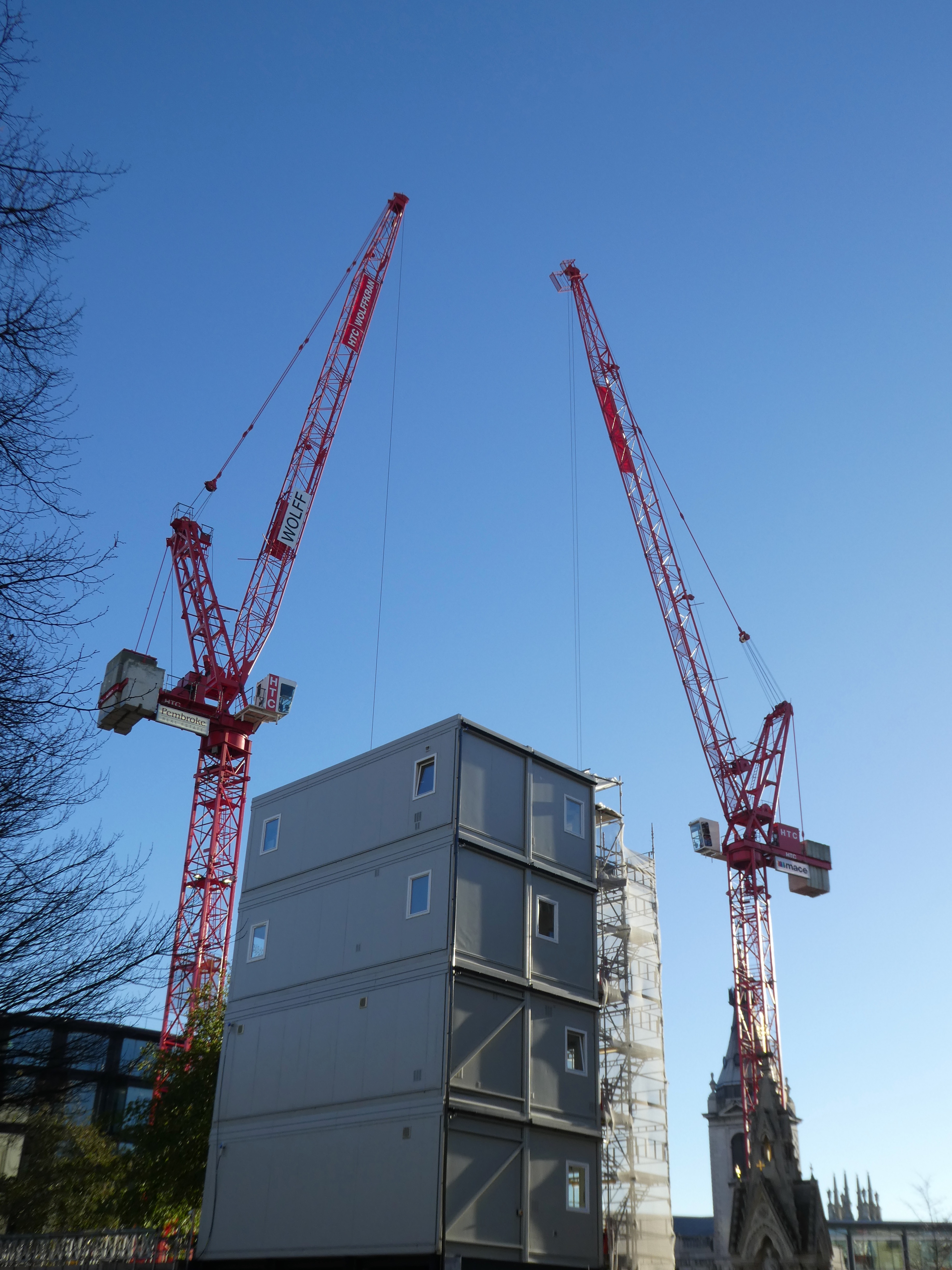
Large mobile cranes can reach up to 700 feet (Figure 2.3.1). This is about the same height as a 50 story building. At such heights, cranes are susceptible to winds and the end of the boom can move back and forth several feet even in moderate winds. We can model the motion as a harmonic oscillator if the side-to-side motion is not too great. However, if the wind becomes too strong and the crane moves too much, gravity will become a factor and the crane may topple due to its weight.
Before we can construct a model that might best describe the swaying of a large crane, we should remind ourselves of how harmonic oscillators work (see Section 1.1). A simple mass-spring system can be modeled by the equation
\begin{equation*}
m \frac{d^2 x}{dt^2} = - kx,
\end{equation*}
where \(x = x(t)\) is the displacement of the mass at time \(t\text{.}\) Given such a system, the mass will oscillate forever with constant amplitude. If we want to be a bit more realistic, we can introduce a damping force,
In the case of our swaying crane, we will let \(x = x(t)\) be the displacement of the end of the boom from the perfect vertical position. When \(x(t) \neq 0\text{,}\) the boom is bent, and the structure of the boom supplies a strong restorative force to bring everything back to a true vertical position. Thus, the swaying of our crane’s boom might be described by an equation such as
The constants \(c_1\) and \(c_2\) can be determined if we know the initial position and initial velocity of the end of the crane’s boom. We show several solutions to our equation in Figure 2.3.2.
Modeling the swaying motion of a crane with a harmonic oscillator might work only if the side-to-side motion is small. If the motion is larger, we must account for the effect of gravity in our model. When \(x(t)\) is large, part of the crane will not be above any other part of the crane. Thus, gravity will pull downward on that part of the crane and will cause the crane to bend even further. We can model this effect by setting the equation for our harmonic oscillator equal to a factor of \(x^3\text{,}\)
When \(x\) is small, this forcing term will not contribute much to the motion of the crane. However, when \(x\) is large, the term will contribute a great deal. The equation \(x'' + 0.1 x' + 0.3 x = 0.02 x^3\) is an example of Duffing’s equation.
The system of equations (2.3.2)–(2.3.3) is nonlinear due the \(x^3\) term. There is little hope to finding an analytic solution to such a system. We can use software to plot the phase plane in order to learn something about the solutions (Figure 2.3.3). However, we still need to numerically generate solutions in order to plot the phase plane.
where \({\mathbf x} = (x, y)\text{,}\)\(d{\mathbf x}/dt = (dx/dt, dy/dt)\text{,}\)\({\mathbf f} = (f, g)\text{,}\) and \({\mathbf x}_0 = (x_0, y_0)\text{.}\) We wish to find approximate values \(x_1, x_2, \ldots, x_n\) and \(y_1, y_2, \ldots, y_n\) for the solution \(x(t)\) and \(y(t)\) at the points
\begin{equation*}
t_k = t_0 + kh, \qquad k = 1, 2, \ldots, n,
\end{equation*}
where \(h\) is the step size. If we let \({\mathbf x}_k = (x_k, y_k)\) and \({\mathbf f}_k = (f(x_k, y_k ), g(x_k, y_k ))\text{,}\) then Euler’s method now becomes
The initial conditions are used to determine \({\mathbf f}_0\text{,}\) which is the tangent vector to the graph of the solution \(\mathbf x(t)\) in the \(xy\)-plane (Figure 2.3.3). We can move in the direction of this tangent vector for time \(h\) in order to find the next point \({\mathbf x}_1\text{.}\) We then calculate a new tangent vector \({\mathbf f}_1\) and then move along this new vector for a time step \(h\) to find \({\mathbf x}_2\text{.}\) We can repeat this technique to generate an approximate solution curve in the phase plane.
with initial conditions \((t_0, x_0, v_0) = (0, 0, 1.7669)\text{.}\) Using a numerical algorithm, we can generate enough points to generate a graph of the solution (Figure 2.3.5).
The surprising thing about Duffing’s equation is that it is extremely sensitive to initial conditions. A slight change in the initial conditions can yield dramatically different solutions. If we change the initial velocity to \(v(0) = 1.7670\text{,}\) we obtain a very different graph of the solution (Figure 2.3.5 ). For small initial velocities, solutions spiral towards the origin. However, a larger initial velocity will send the solution in the phase plane away from the origin. If the crane sways too violently, we will have a disaster.
Notice that our system is not autonomous and depends on time. Therefore, we cannot graph the phase plane of this system; however, we can graph a solution curve in three dimensions (Figure 2.3.9).
Use Euler’s method with step size \(\Delta t = 0.5\) to approximate this solution, and check how close the approximation is to the real solution when \(t = 2\text{,}\)\(t = 4\text{,}\) and \(t = 6\text{.}\)
Use Euler’s method with step size \(\Delta t = 0.1\) to approximate this solution, and check how close the approximation is to the real solution when \(t = 2\text{,}\)\(t = 4\text{,}\) and \(t = 6\text{.}\)
Just as in the case of a single first-order differential equation, we can think of Euler’s approximation as the first two terms of the Taylor series expansion,
To get a more accurate approximation, we can take the first two terms of the Taylor series. In this case, we must compute \({\mathbf x}''\text{.}\) If we return to our example,
be a system of differential equations such that \({\mathbf f}\) is continuously differentiable. If \({\mathbf x}_0\) is the initial value at time \(t_0\text{,}\) there exists a unique solution for the initial value problem on some open interval \(t_0 - \epsilon \lt t \lt t_0 + \epsilon\) for some \(\epsilon > 0\text{.}\)
If we have an autonomous system \({\mathbf x}' = {\mathbf f}({\mathbf x})\text{,}\) our solution does not depend on time. Thus, we obtain the same solution curve if we start at the same point even though we might start at different times.
Many systems of equations cannot be solved analytically. However, we can use numerical techniques such as Euler’s Method to find approximate solutions for the system. Given the system
Provided certain conditions are met, we are guaranteed unique local solutions to any system of first-order differential equations. Some of the following are consequences of existence and uniqueness.
If we have an autonomous system \({\mathbf x}' = {\mathbf f}({\mathbf x})\text{,}\) our differential equation does not depend on time. Thus, we obtain the same solution curve if we start at the same point even though we might start at different times.
Use Euler’s method with step size \(\Delta t = 0.5\) to approximate this solution, and check how close the approximation is to the real solution when \(t = 2\text{,}\)\(t = 4\text{,}\) and \(t = 6\text{.}\)
Use Euler’s method with step size \(\Delta t = 0.1\) to approximate this solution, and check how close the approximation is to the real solution when \(t = 2\text{,}\)\(t = 4\text{,}\) and \(t = 6\text{.}\)